plotnine
plotnine is a Python implementation of the grammar of graphics, built by Hassan Kibirige and a community of contributors to track R’s ggplot2 as closely as the two languages allow. If you already think in ggplot() + geom_*() + facet_*() + theme_*(), plotnine gives you that exact mental model in Python: layered geoms, statistical transforms, scales, faceting, and a rich theming system, all composable with +. Since version 0.15 it also supports compositions – arranging whole plots next to and above one another with | and /, the same operators patchwork popularized in R.
Shiny for Python can already show a plotnine plot with the built-in @render.plot: it calls .draw() and sends back a static PNG. @render_plotnine (pip install 'shinywidgets[plotnine]') instead draws the plot once to a live ipympl canvas that stays on the server for as long as the output is displayed. That gets you a few things a static image can’t: the matplotlib toolbar (zoom, pan, home, back/forward, PNG download) for free, a clicked() accessor that turns a mouse press into a reactive value, a limits() accessor that turns the current zoom window into a reactive value you can read anywhere, and the ability to edit the rendered figure’s artists in place without a full re-render. It also renders compositions, which @render.plot rejects outright. The trade-off is cost and limits: every interaction redraws the figure in Python and ships a new image over the websocket, so it doesn’t scale to huge datasets or brush-to-select the way @render.plot’s built-in brush=True does, and because render_plotnine reuses the generic ipympl canvas, there’s no click-to-facet or click-to-data-value translation built in – you do that mapping yourself (shown below).
render_plotnine shares its rendering machinery and two of matplotlib’s three accessors, clicked() and limits(), with render_matplotlib – both coerce to the same ipympl.backend_nbagg.Canvas widget. If your plot doesn’t need plotnine’s grammar (you’re building a figure directly with matplotlib, pandas’ .plot(), or seaborn), use the matplotlib guide instead; the toolbar, in-place update, and accessor material there applies unchanged. Reach for render_plotnine here when ggplot syntax is how you already build the plot, and reach for @render.plot when the plot is just a picture: large data, a dashboard with many small static plots, or brush selection (see the comparison in Gotchas and limitations).
Installation
pip install 'shinywidgets[plotnine]'This installs plotnine and ipympl (the live-canvas backend render_plotnine draws to). No JavaScript bundle to configure – ipympl ships its own.
Quick start
from plotnine import aes, geom_point, geom_smooth, ggplot, labs, theme_minimal
from plotnine.data import mpg
from shiny.express import ui
from shinywidgets import render_plotnine

ui.page_opts(title="plotnine quick start", fillable=True)

with ui.card(full_screen=True):
    ui.card_header("Engine displacement vs. highway MPG")

    @render_plotnine
    def plot():
        return (
            ggplot(mpg, aes("displ", "hwy", color="class"))
            + geom_point(size=2.5, alpha=0.8)
            + geom_smooth(method="lm", color="black", se=False)
            + labs(x="Displacement (L)", y="Highway MPG", color="Class")
            + theme_minimal()
        )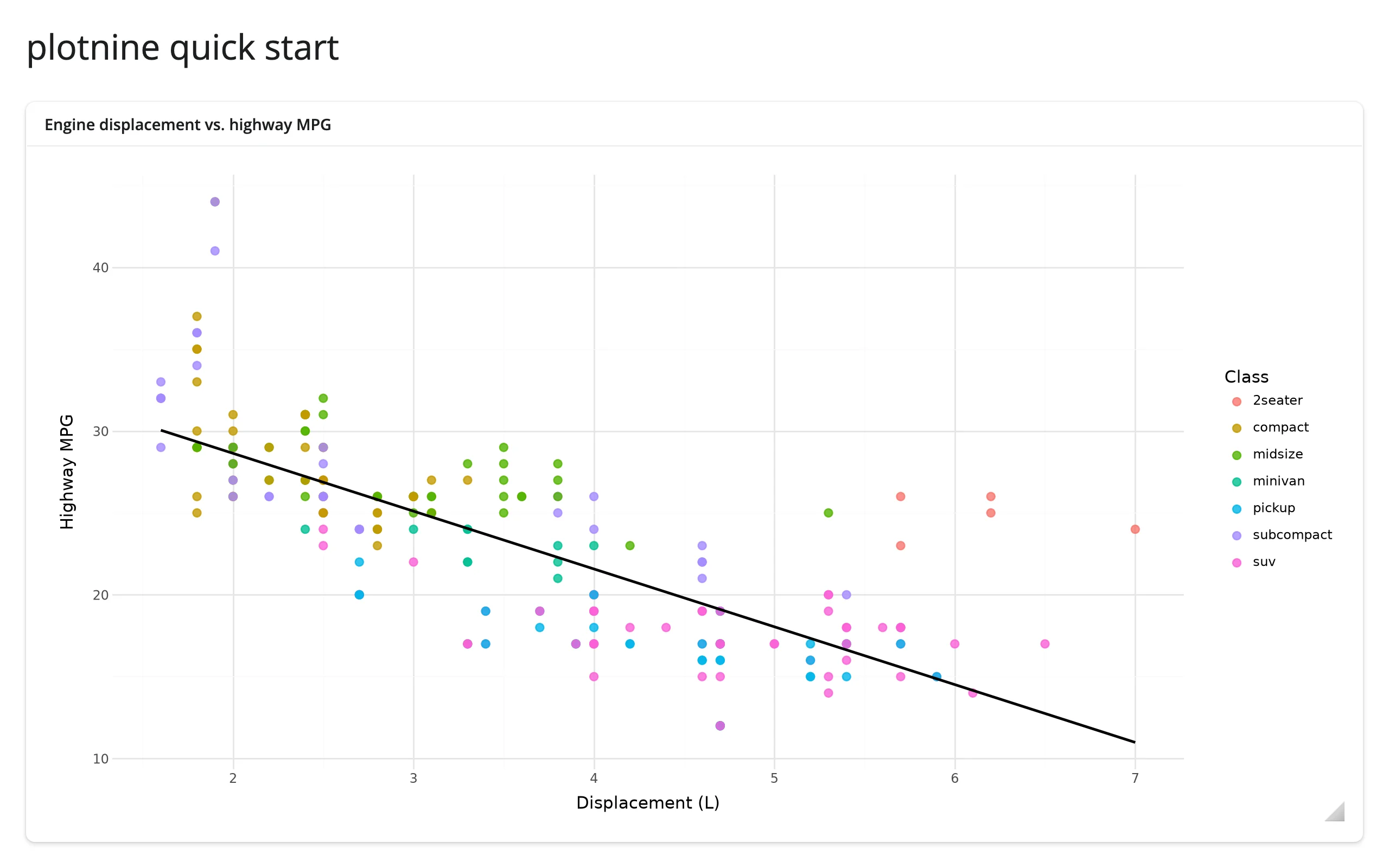
Return a ggplot from the decorated function the same as you would from a notebook cell. render_plotnine draws it (a copy – your plot object is never mutated), resizes the figure to fill the card, and plotnine re-runs its own layout engine (legend, axis labels, facet strips) every time the card resizes. Hover the plot and a toolbar fades in at the top-left with zoom, pan, home/back/forward, and PNG download – see What you can build.
What you can build
Plot compositions, not just single plots
from plotnine import aes, geom_boxplot, geom_histogram, geom_point, ggplot, labs, theme
from plotnine.data import penguins
from shiny.express import ui
from shinywidgets import render_plotnine

penguins = penguins.dropna().reset_index(drop=True)

ui.page_opts(title="plotnine compositions", fillable=True)

no_legend = theme(legend_position="none")

with ui.card(full_screen=True):
    ui.card_header("Bill shape, species, and flipper length")

    @render_plotnine
    def composed():
        scatter = (
            ggplot(penguins, aes("bill_length_mm", "bill_depth_mm", color="species"))
            + geom_point()
            + labs(x="Bill length (mm)", y="Bill depth (mm)", color="Species")
        )
        box = (
            ggplot(penguins, aes("species", "body_mass_g", fill="species"))
            + geom_boxplot()
            + labs(x="", y="Body mass (g)")
            + no_legend
        )
        hist = (
            ggplot(penguins, aes("flipper_length_mm", fill="species"))
            + geom_histogram(bins=30, alpha=0.7, position="identity")
            + labs(x="Flipper length (mm)", y="Count")
            + no_legend
        )
        return (scatter | box) / hist
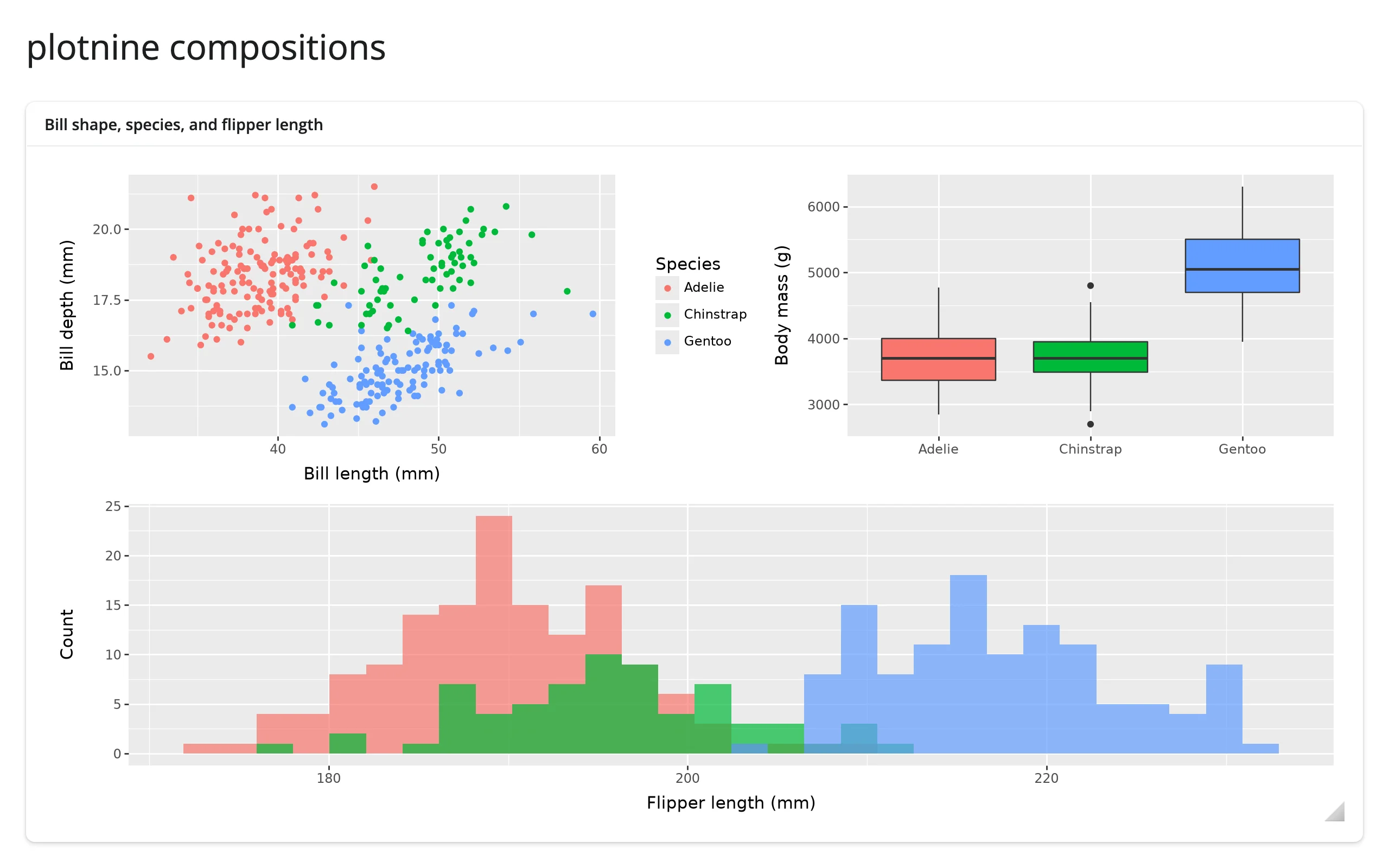
(scatter | box) / hist lays the three plots out as one figure – a scatter and a box plot side by side, a histogram underneath – and render_plotnine treats the whole thing as a single widget: one toolbar, one resize target, re-laid out as a unit. @render.plot can’t display this at all: it raises @render.plot doesn't know to render objects of type '<class 'plotnine.composition._beside.Beside'>' (verified). This is the most direct reason to reach for render_plotnine over the static renderer when a dashboard panel needs more than one related plot.
A toolbar for free: zoom, pan, home, download
from plotnine import aes, geom_line, ggplot, labs, theme_minimal
from plotnine.data import economics
from shiny.express import ui
from shinywidgets import render_plotnine

ui.page_opts(title="Zoom and pan, no extra code", fillable=True)

with ui.card(full_screen=True):
    ui.card_header("US unemployment, 1967-2015 -- hover to reveal the toolbar")

    @render_plotnine
    def plot():
        return (
            ggplot(economics, aes("date", "unemploy"))
            + geom_line()
            + labs(x="", y="Unemployed (thousands)")
            + theme_minimal()
        )
Before and after dragging the “zoom to rectangle” tool over the 1998-2008 stretch:
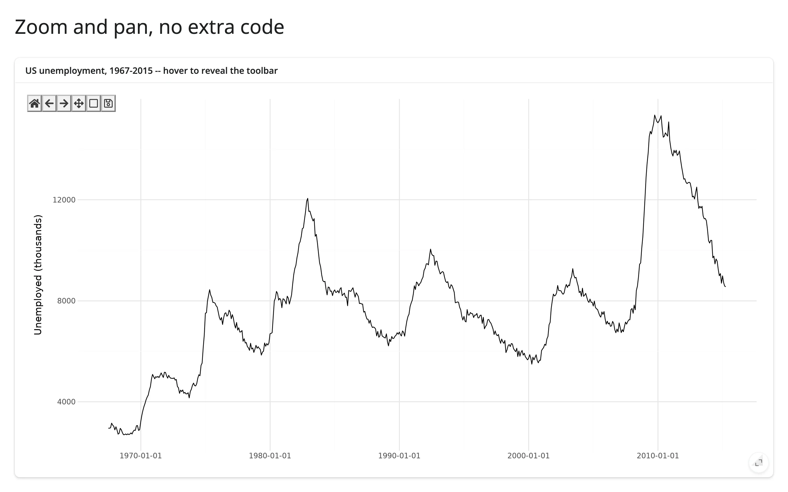
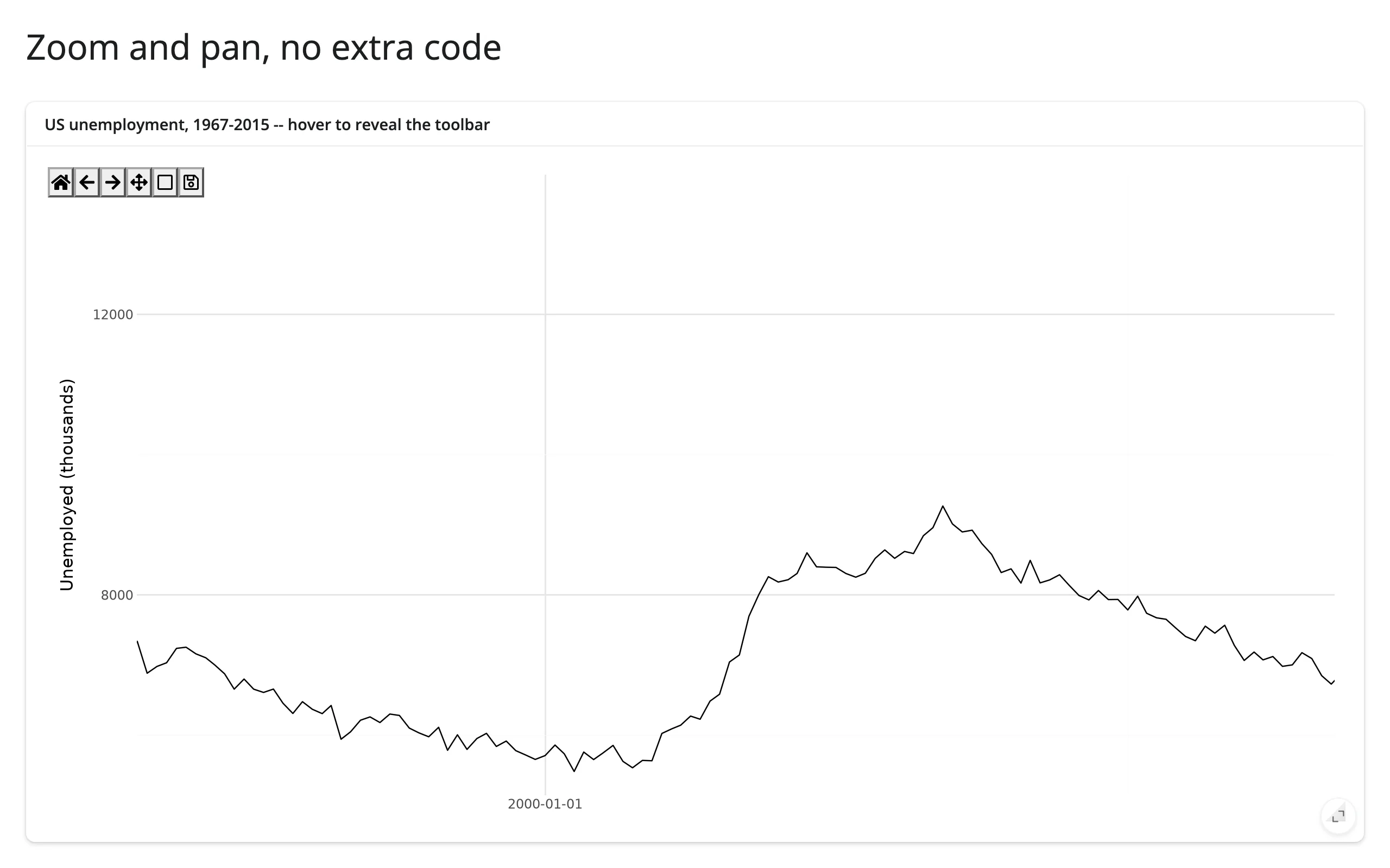
No code beyond the plot itself: render_plotnine always wires up ipympl’s toolbar (box zoom, pan with left/right mouse buttons, home, back/forward view history, and PNG download). You don’t write any of this; you only need code once you want Python to react to it (see Reacting to user interaction). Notice the zoomed-in x-axis in the second screenshot: it shows only one date tick. That’s plotnine’s axis breaks, computed once at draw time – see Gotchas and limitations for the fix.
Facets and themes that relayout live
from plotnine import aes, facet_wrap, geom_point, ggplot, labs, theme_light
from plotnine.data import mpg
from shiny.express import ui
from shinywidgets import render_plotnine

ui.page_opts(title="Facets that relayout live", fillable=True)

with ui.card(full_screen=True):
    ui.card_header("Highway MPG by displacement, faceted by drivetrain")

    @render_plotnine
    def plot():
        return (
            ggplot(mpg, aes("displ", "hwy", color="class"))
            + geom_point(size=2)
            + facet_wrap("~drv", labeller="label_both")
            + labs(x="Displacement (L)", y="Highway MPG", color="Class")
            + theme_light()
        )
Wide and narrow (resized to a 650px-wide card):
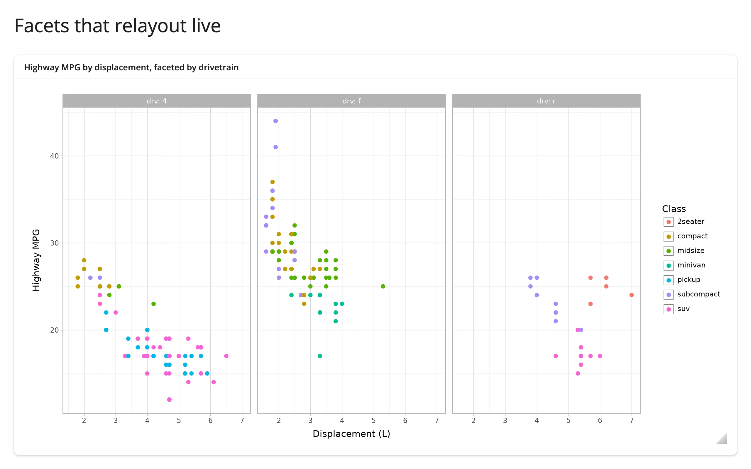
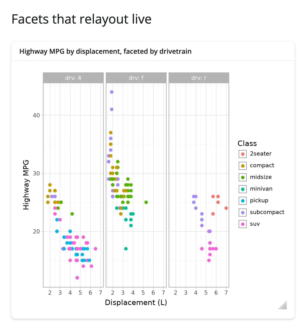
Every resize – dragging the window, collapsing a sidebar, entering full_screen – triggers a real plotnine redraw, not a CSS rescale. Facet strips, legend placement, and axis label wrapping are recomputed at the new size, the same as they would be if you called .draw() again at a different figure_size. This is what theme(dpi=...) and theme(figure_size=...) would otherwise need you to pick in advance for a static image.
Reacting to user interaction
Accessor reference
| accessor | returns | before any interaction | across re-render | default rate policy |
|---|---|---|---|---|
clicked() |
matplotlib.backend_bases.MouseEvent |
None |
kept (payload describes the previous render’s figure) | not rate-limited |
limits(ax=0) |
((x0, x1), (y0, y1)) for panel ax |
seeded value (the figure’s rendered limits) | re-seeded from the new figure | debounced, 250 ms |
Both are the same underlying accessors as render_matplotlib (both renderers coerce to the same ipympl Canvas), documented separately here because the coordinate space is plotnine’s own: .xdata/.ydata and limits()’s bounds are in plotnine’s transformed units, not necessarily the values in your data frame (see below). clicked() attaches the moment the figure renders and keeps its value across a re-render until the user clicks the new figure; limits() instead re-seeds from the new figure’s own limits on every render, since it describes the figure’s current view rather than something the user did. A press that starts a toolbar pan/zoom drag, or lands outside every axes (e.g., in the legend), doesn’t count toward clicked(). A double-click arrives as three separate presses – MouseEvent has no equality, so repeats are never deduplicated.
render_matplotlib also has picked(); plotnine doesn’t get it. plotnine’s geoms reject matplotlib’s picker= kwarg outright (geom_point(picker=5) raises PlotnineError: Parameters {'picker'} ... are not understood, verified), so no plotnine artist can ever be made pickable – picked() would just never fire.
clicked(): the nearest point, as a reactive value
import numpy as np
from plotnine import aes, geom_point, ggplot, labs, theme_minimal
from plotnine.data import mpg
from shiny import reactive, req
from shiny.express import render, ui
from shinywidgets import render_plotnine

ui.page_opts(title="plot.clicked(): nearest point", fillable=True)
nearest = reactive.value(None)

with ui.layout_columns():
    with ui.card(full_screen=True):

        @render_plotnine
        def plot():
            return (
                ggplot(mpg, aes("displ", "hwy"))
                + geom_point(size=2.5, alpha=0.7)
                + labs(x="Displacement (L)", y="Highway MPG")
                + theme_minimal()
            )

    with ui.card():
        ui.card_header("Clicked car")

        @render.ui
        def detail():
            # Compare to None explicitly: a row position of 0 is falsy, so
            # req(nearest()) would wrongly treat that valid click as "no click"
            i = nearest()
            if i is None:
                return ui.p("Click a point to see that car here.")
            row = mpg.iloc[i]
            return ui.p(
                f"{row.manufacturer.title()} {row.model}: {row.displ} L, {row.hwy} MPG hwy"
            )


@reactive.effect
def _mark_nearest():
    event = plot.clicked()
    canvas = plot.widget
    req(event, canvas)
    ax = canvas.figure.axes[0]
    xy = ax.transData.transform(mpg[["displ", "hwy"]].to_numpy())
    i = int(np.hypot(xy[:, 0] - event.x, xy[:, 1] - event.y).argmin())
    nearest.set(i)

    for artist in list(ax.lines):
        if artist.get_label() == "_clicked":
            artist.remove()
    row = mpg.iloc[i]
    ax.plot(
        [row.displ],
        [row.hwy],
        "o",
        ms=14,
        mfc="none",
        mec="black",
        mew=2,
        label="_clicked",
    )
    canvas.draw_idle()
Before any click, and after clicking near the middle of the cloud:
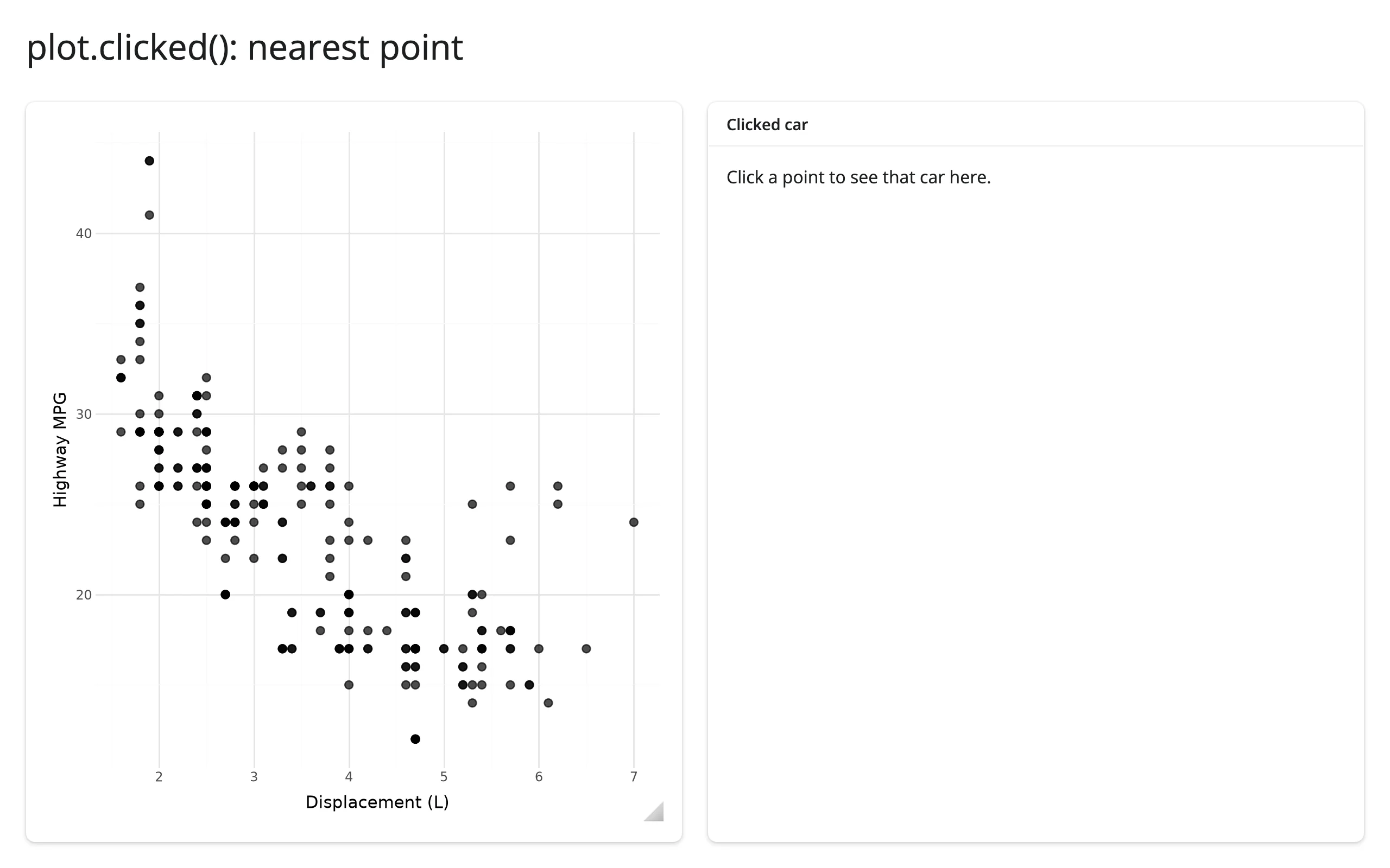
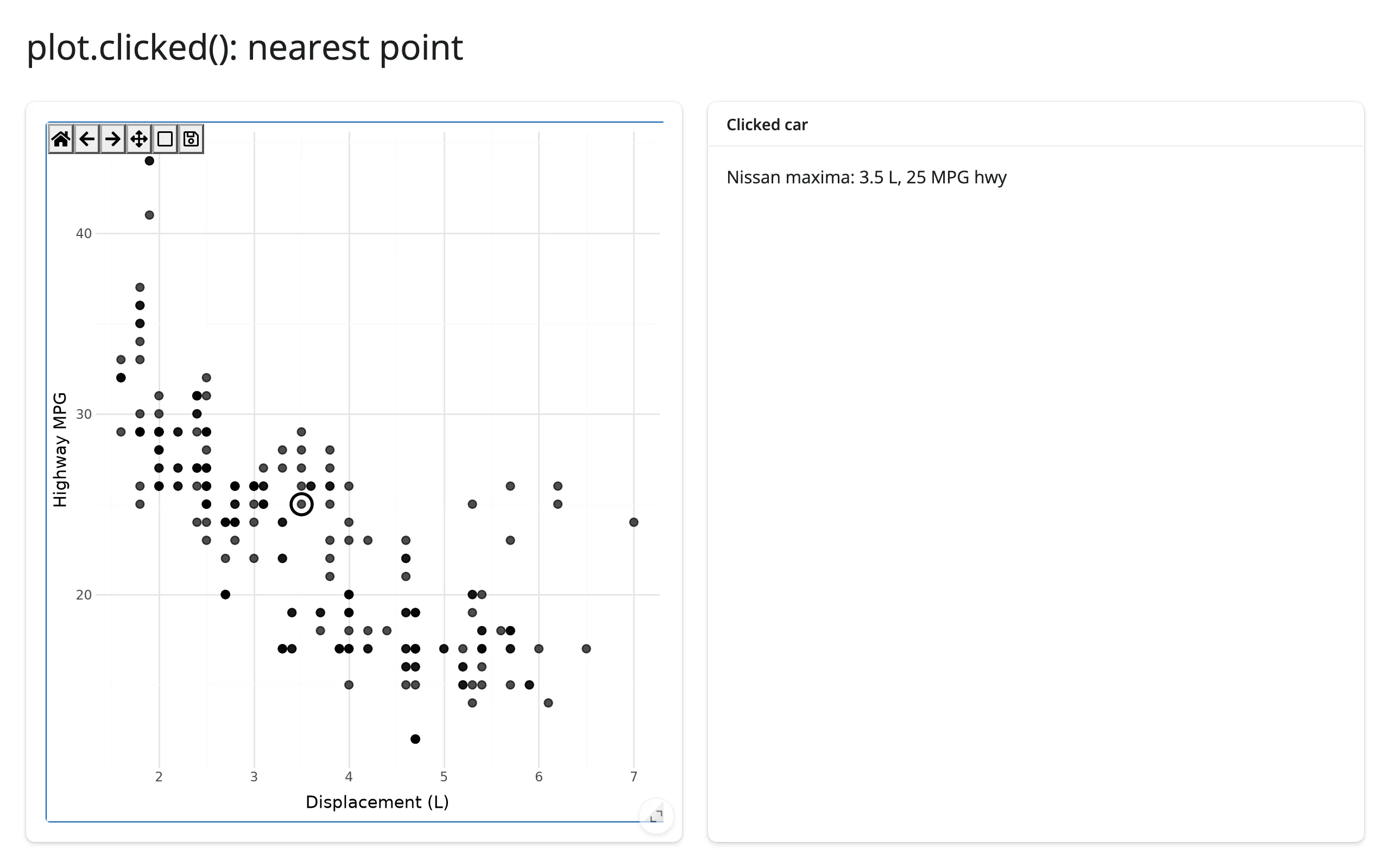
clicked() gives you a raw MouseEvent, not a row – there’s no “nearest point” built in, because plotnine doesn’t keep a mapping from pixels back to your data frame. The standard recipe is: transform your data’s x/y columns to display (pixel) coordinates with ax.transData.transform(...), then compare against event.x / event.y (also in display coordinates) with a plain nearest-neighbor search. Comparing in display space, rather than data space, avoids unit mismatches when x and y have very different scales. The effect reads both plot.clicked() (the dependency that makes it re-run on each press) and plot.widget (the current canvas) so it can draw a circle around the match directly on the figure – see Updating the widget from Python for why editing the canvas in place, instead of returning a new plot, is what keeps the circle and the user’s current zoom level both visible at once. clicked() attaches at render and keeps its value across a re-render (the payload then refers to the previous render’s figure), so prefer an ID-keyed lookup over a positional row index if your underlying data can change shape between renders.
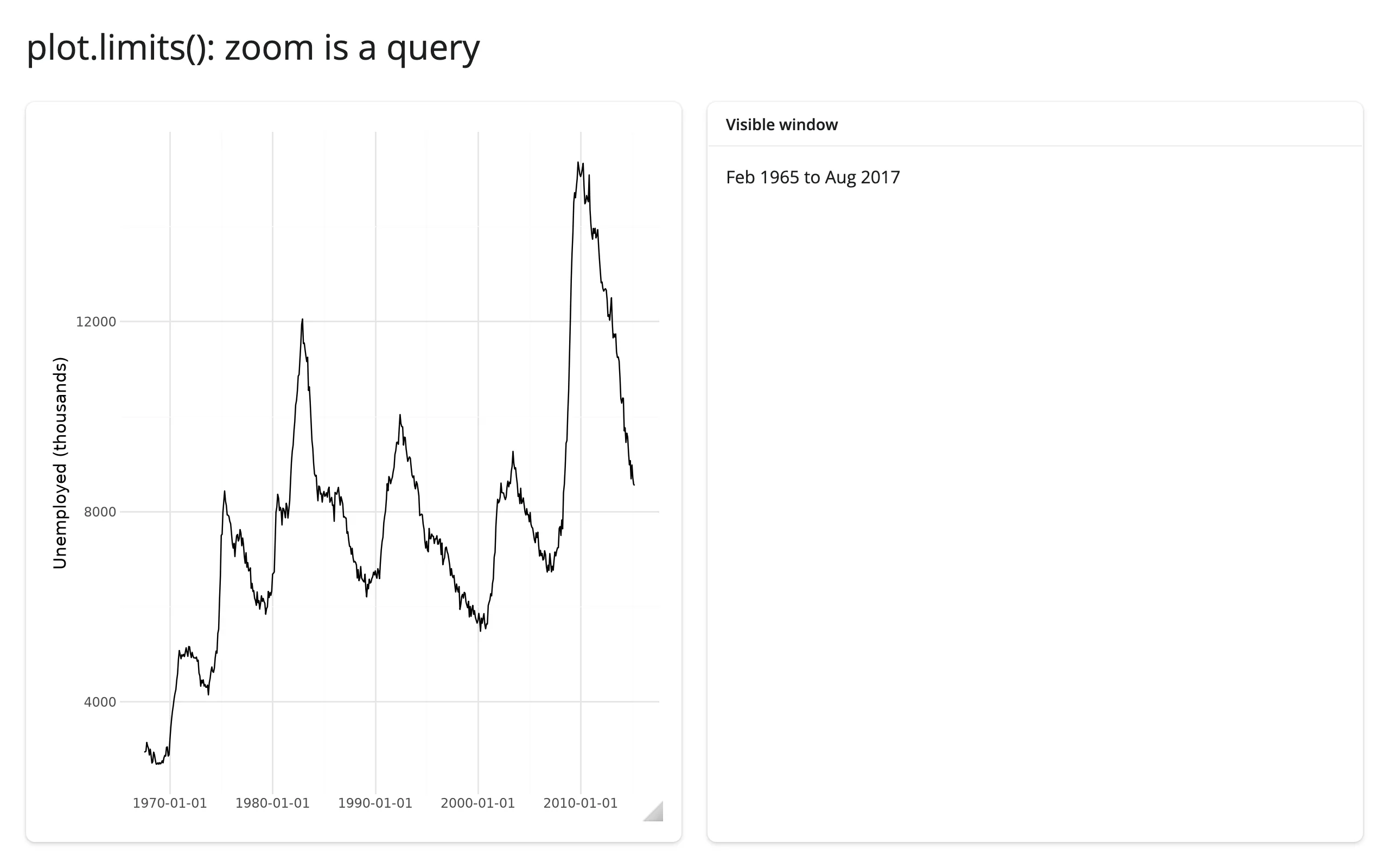
limits(): zoom is a query
import matplotlib.dates as mdates
from plotnine import aes, geom_line, ggplot, labs, theme_minimal
from plotnine.data import economics
from shiny.express import render, ui
from shinywidgets import render_plotnine

ui.page_opts(title="plot.limits(): zoom is a query", fillable=True)

with ui.layout_columns():
    with ui.card(full_screen=True):

        @render_plotnine
        def plot():
            return (
                ggplot(economics, aes("date", "unemploy"))
                + geom_line()
                + labs(x="", y="Unemployed (thousands)")
                + theme_minimal()
            )

    with ui.card():
        ui.card_header("Visible window")

        @render.text
        def window():
            (x0, x1), _ = plot.limits()
            # x0/x1 are plotnine's *transformed* x values -- here matplotlib's
            # date-number epoch, not a datetime -- convert to read them
            lo, hi = mdates.num2date(x0), mdates.num2date(x1)
return f"{lo:%b %Y} to {hi:%b %Y}"| Before zoom | After zoom |
|---|---|
 |
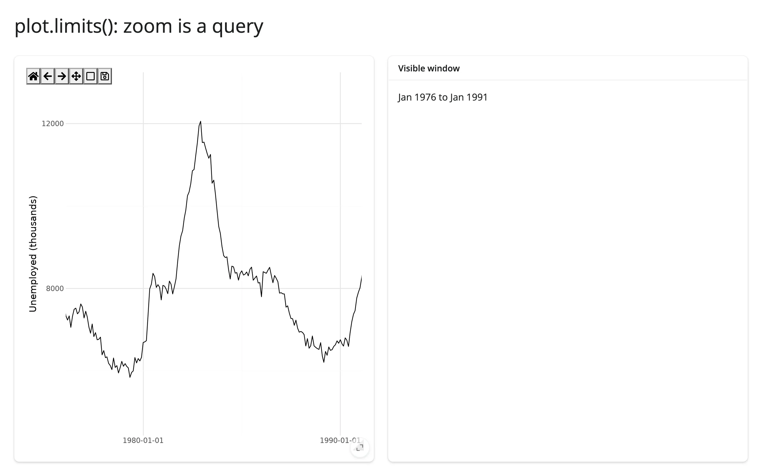 |
limits() is seeded from the figure’s rendered limits, then updates (debounced 250 ms) after every zoom or pan step. Like clicked(), the values are in plotnine’s transformed coordinate space: here they’re matplotlib’s date-number epoch, so reading them as a real date needs matplotlib.dates.num2date(), same as clicked()’s .xdata would under a scale_x_log10() plot (10 ** x recovers the data value). It can’t be read inside the plot’s own render function, which builds a new figure every run – read it in another output or an effect instead. Unlike clicked(), a re-render re-seeds limits() from the new figure’s own view rather than carrying over the old zoom window.
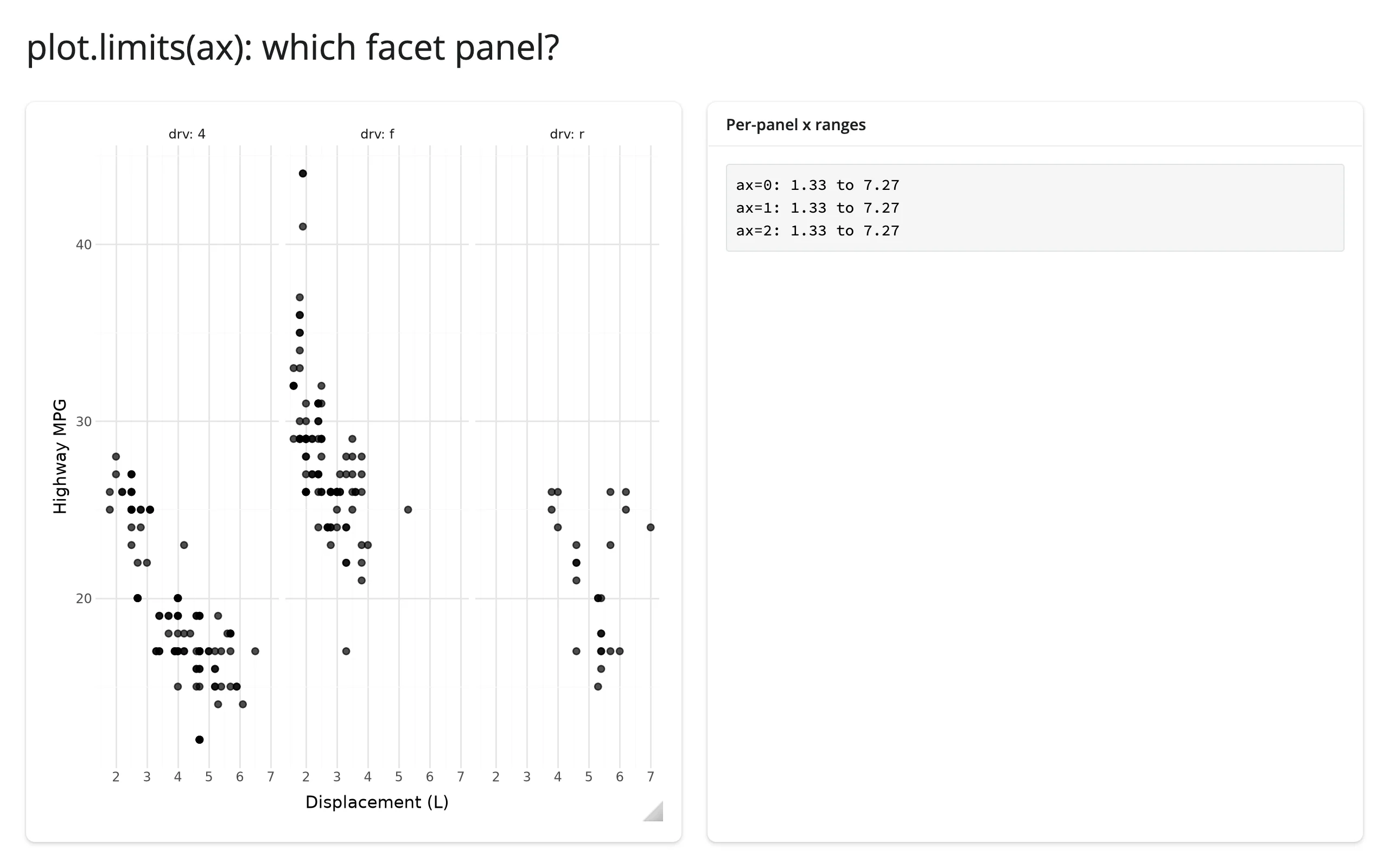
ax indexes panels: with facet_wrap()/facet_grid(), limits(ax=1) reads the second facet panel’s own x/y range, in the same order as .widget.figure.axes.
from plotnine import aes, facet_wrap, geom_point, ggplot, labs, theme_minimal
from plotnine.data import mpg
from shiny.express import render, ui
from shinywidgets import render_plotnine

ui.page_opts(title="plot.limits(ax): which facet panel?", fillable=True)

with ui.layout_columns():
    with ui.card(full_screen=True):

        @render_plotnine
        def plot():
            return (
                ggplot(mpg, aes("displ", "hwy"))
                + geom_point(size=2, alpha=0.7)
                + facet_wrap("~drv", labeller="label_both")
                + labs(x="Displacement (L)", y="Highway MPG")
                + theme_minimal()
            )

    with ui.card():
        ui.card_header("Per-panel x ranges")

        @render.code
        def ranges():
            n = len(plot.widget.figure.axes)
            lines = []
            for i in range(n):
                x0, x1 = plot.limits(ax=i)[0]
                lines.append(f"ax={i}: {x0:.2f} to {x1:.2f}")
return "\n".join(lines)| Before zoom | After zooming into the drv: 4 panel |
|---|---|
 |
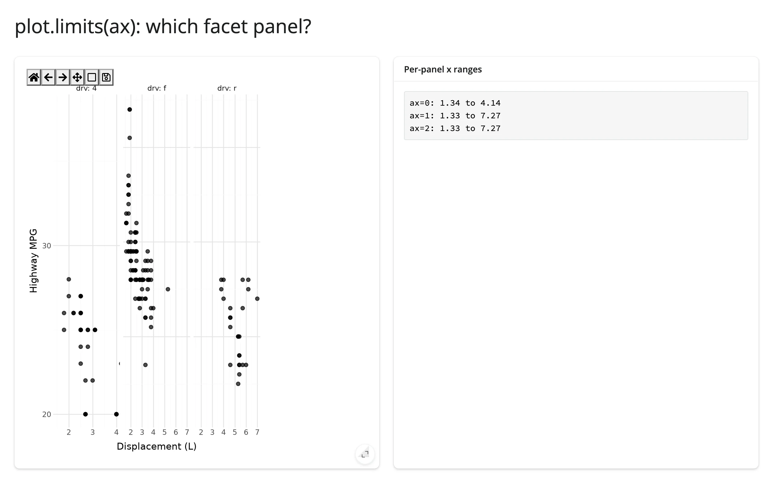 |
Zooming a single facet panel only changes that panel’s own entry – the other two stay at the full range, confirming ax tracks panels independently and in figure.axes order.
Reading an accessor on demand
Because every accessor is live from the moment the figure renders, it’s safe to read one anywhere – a button handler, a download handler, a @reactive.event – not just from an output that’s always on screen. Here, a “Save current view” button reads plot.limits() on click and appends it to a running list, with no warm-up @reactive.effect needed to make the first read work:
from plotnine import aes, geom_point, ggplot, labs, theme_minimal
from plotnine.data import mpg
from shiny import reactive
from shiny.express import input, render, ui
from shinywidgets import render_plotnine

ui.page_opts(title="Save the current zoom window", fillable=True)
ui.input_action_button("save", "Save current view")

bookmarks = reactive.value([])


@render_plotnine
def plot():
    return (
        ggplot(mpg, aes("displ", "hwy", color="class"))
        + geom_point(size=2.5, alpha=0.8)
        + labs(x="Displacement (L)", y="Highway MPG", color="Class")
        + theme_minimal()
    )


@reactive.effect
@reactive.event(input.save)
def _save_view():
    (x0, x1), (y0, y1) = plot.limits()
    bookmarks.set([*bookmarks(), f"x: {x0:.1f}-{x1:.1f}, y: {y0:.1f}-{y1:.1f}"])


@render.code
def saved():
    views = bookmarks()
    if not views:
        return "No views saved yet -- zoom in, then click Save."
    return "\n".join(f"{i + 1}. {v}" for i, v in enumerate(views))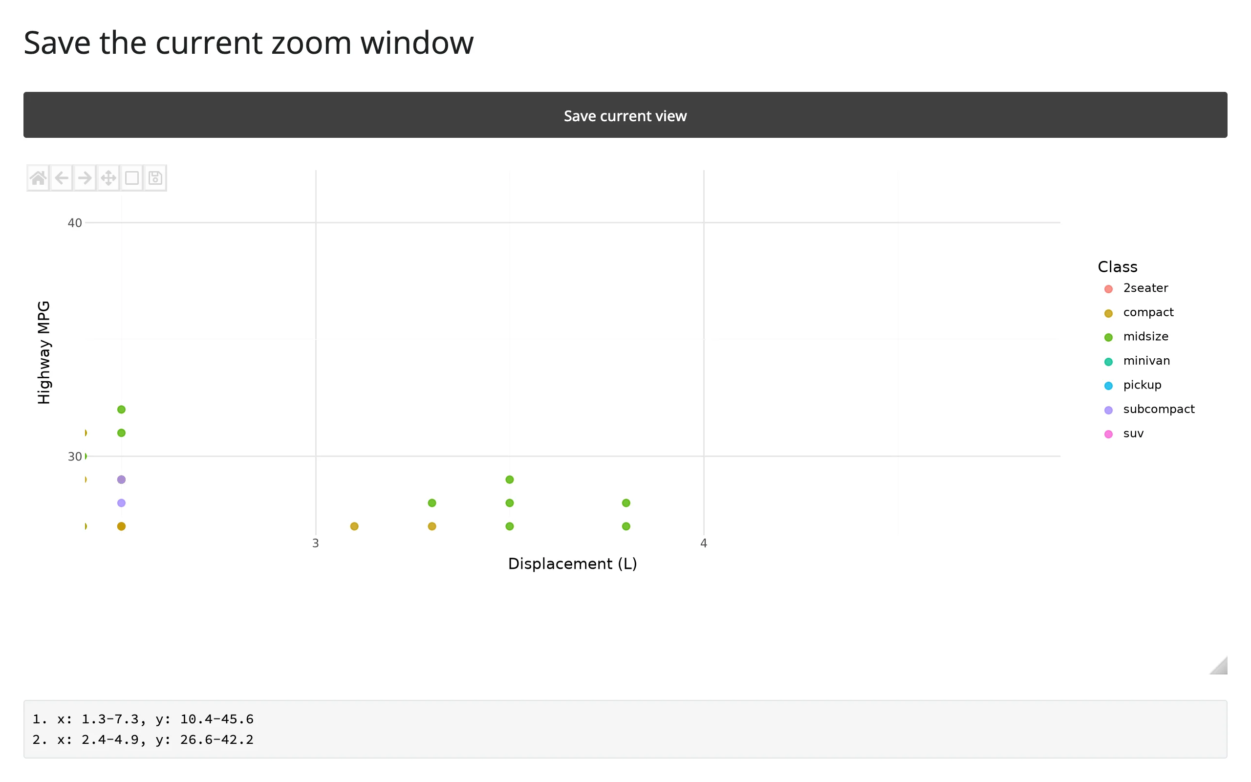
Verified: clicking Save before any zoom records the figure’s full extent (limits() is already seeded, not None); zooming in and clicking Save again appends the new window.
Beyond the accessors: .read() and reactive_read()
plotnine’s canvas has no synced trait for the plot’s current view, so there’s nothing to plot.read(...) (which falls through to reactive_read() for names that aren’t accessors) for “zoom level” the way jupyter-scatter or ipyleaflet expose one – use limits() for that, above. One toolbar trait on the underlying widget is worth reading directly, though, since it’s a child widget of the canvas rather than the output itself:
reactive_read(canvas.toolbar, "_current_action") # '', 'pan', or 'zoom'This tells you whether the user currently has the pan or zoom tool active, e.g., to suppress your own click handling while a drag is in progress (clicked() already does this filtering for you) or to show a status badge. It’s a private ipympl trait (leading underscore), so treat it as liable to change in a future ipympl release. For the view itself (what’s currently visible after a zoom or pan), use limits() – there’s no longer a reason to hand-roll ax.callbacks.connect("xlim_changed", ...) the way earlier versions of this guide did.
Rate limiting
clicked() has no default rate policy: it reports every press immediately, because a click is a discrete event, not a stream. limits() is debounced 250 ms by default – a zoom-to-rectangle drag fires about a dozen xlim_changed events, and only the settled value after the pause reaches Python. Pass rate_delay=0 to react to every event instead (e.g. to drive a second plot smoothly while panning), or rate_policy="throttle" to get evenly-spaced updates during a long drag rather than waiting for it to stop:
from plotnine import aes, geom_line, ggplot, labs, theme_minimal
from plotnine.data import economics
from shiny.express import render, ui
from shinywidgets import render_plotnine

ui.page_opts(fillable=True)

counts = {"default": 0, "fast": 0}


def make_plot():
    return (
        ggplot(economics, aes("date", "unemploy"))
        + geom_line()
        + labs(x="", y="Unemployed (thousands)")
        + theme_minimal()
    )


with ui.layout_columns():
    with ui.card():
        ui.card_header("default: debounced 250ms")

        @render_plotnine
        def default_out():
            return make_plot()

        @render.code
        def default_count():
            default_out.limits()
            counts["default"] += 1
            return f"limits() recomputed {counts['default']} times"

    with ui.card():
        ui.card_header("rate_delay=0: every event")

        @render_plotnine(rate_delay=0)
        def fast_out():
            return make_plot()

        @render.code
        def fast_count():
            fast_out.limits()
            counts["fast"] += 1
            return f"limits() recomputed {counts['fast']} times"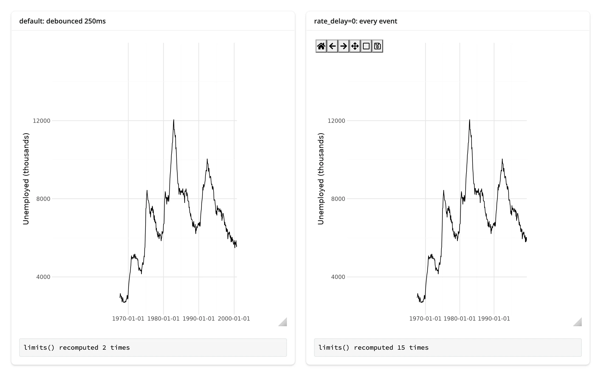
Panning the same distance on both plots (verified with a scripted drag): the debounced plot recomputed twice (the initial seed, then the settled value), the rate_delay=0 plot recomputed 15 times. rate_policy/rate_delay also apply to reactive_read() on .widget, same as every renderer in this roster, but limits() is the only accessor here a rate policy actually changes.
Updating the widget from Python
Two ways to change a plot that’s already on screen:
- Re-render (return a new
ggplotfrom the decorated function): simplest, and the only option when the underlying data actually changes shape. plotnine draws an entirely new figure, so the user’s zoom, pan position, and any artists you added (like the circle marker above) are all lost. - Update in place, from a
@reactive.effectthat reads.widgetand edits the matplotlibAxesdirectly (ax.lines[i].set_ydata(...), add an artist, etc.), then callscanvas.draw_idle(): the figure keeps its current zoom and pan, and nothing is re-sent except the one redrawn frame.
plotnine itself has no “replace this layer’s data” API the way plotly or bokeh do – a ggplot object isn’t mutable in that sense. In-place updates to a plotnine-drawn figure mean reaching past plotnine into the matplotlib artists it produced, the same technique render_matplotlib documents. The one plotnine-specific wrinkle: which artist is “the line” depends on your geoms and draw order (ax.lines[0] for a single geom_line, ax.collections[0] for a single geom_point), and that index isn’t guaranteed stable if you add or remove layers – inspect ax.lines/ax.collections once on a drawn figure to find the index you need.
examples/07_update_inplace.py contrasts the two side by side: a frequency slider redraws the left plot from scratch each time, while the right plot is built once and only has its line’s y data replaced.
import numpy as np
import pandas as pd
from plotnine import aes, geom_line, ggplot, scale_y_continuous, theme_minimal
from shiny import reactive
from shiny.express import input, ui
from shinywidgets import render_plotnine

ui.page_opts(title="Re-render vs. in-place", fillable=True)
ui.input_slider("freq", "Frequency", 1, 10, 3)

x = np.linspace(0, 1, 400)


def wave(freq: int) -> pd.DataFrame:
    return pd.DataFrame({"x": x, "y": np.sin(2 * np.pi * freq * x)})


with ui.layout_columns():
    with ui.card(full_screen=True):
        ui.card_header("Re-render: zoom resets")

        @render_plotnine
        def rerendered():
            return (
                ggplot(wave(input.freq()), aes("x", "y"))
                + geom_line()
                + scale_y_continuous(limits=(-1.1, 1.1))
                + theme_minimal()
            )

    with ui.card(full_screen=True):
        ui.card_header("In-place: zoom survives")

        @render_plotnine
        def inplace():
            # Doesn't read input.freq(): built once, edited afterward
            return (
                ggplot(wave(3), aes("x", "y"))
                + geom_line()
                + scale_y_continuous(limits=(-1.1, 1.1))
                + theme_minimal()
            )


@reactive.effect
def _update_wave():
    freq = input.freq()
    with reactive.isolate():
        canvas = inplace.widget
    if canvas is None:
        return
    line = canvas.figure.axes[0].lines[0]
    line.set_ydata(np.sin(2 * np.pi * freq * x))
    canvas.draw_idle()
Both plots zoomed to the same window, then the frequency slider moved to 8:
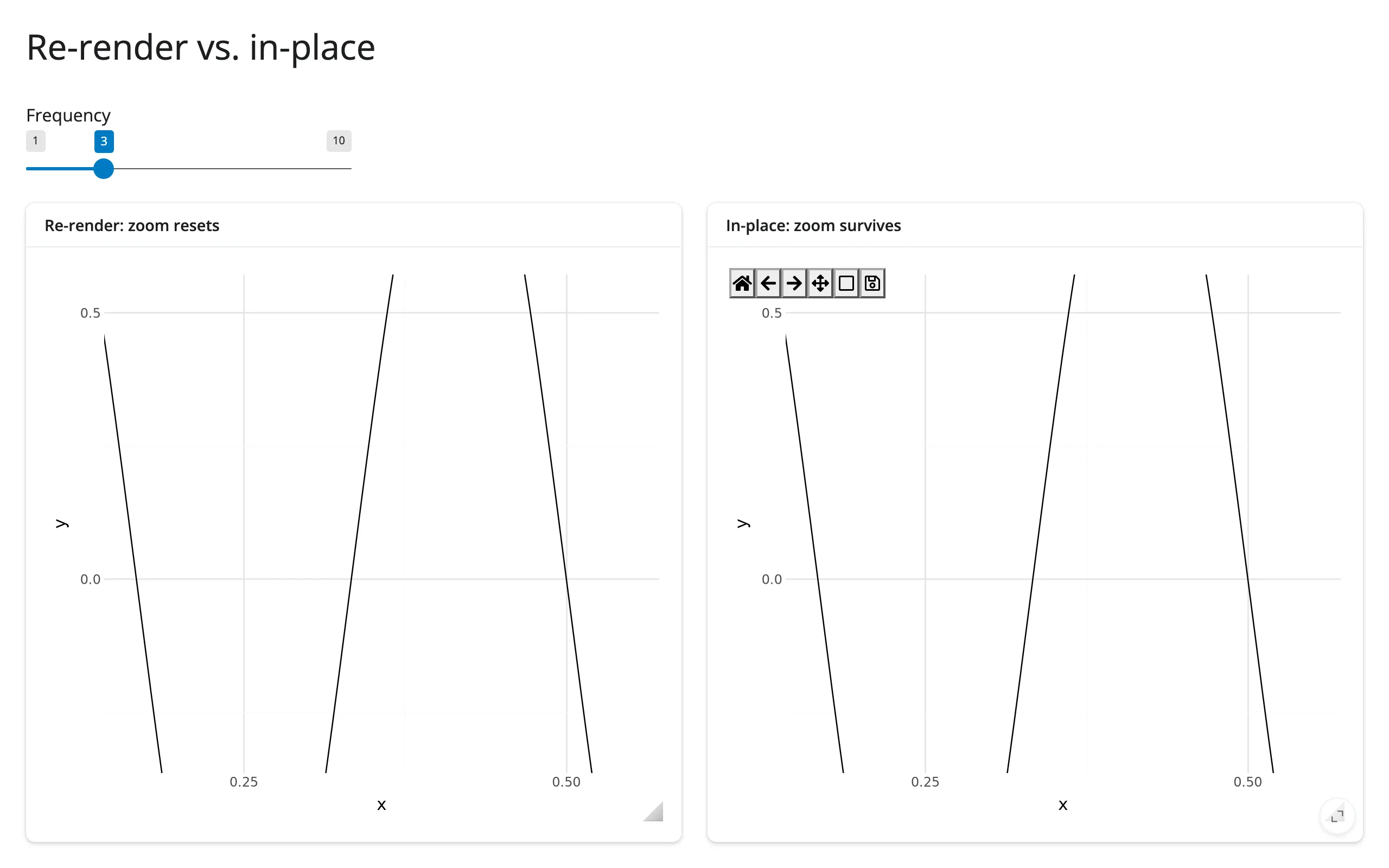
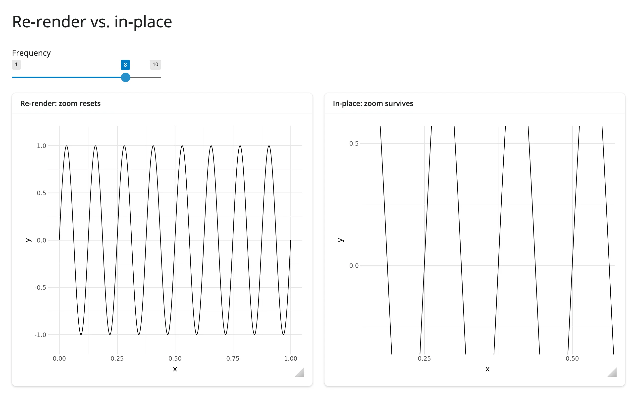
The re-rendered plot (left) snapped back to showing the full x-axis and lost the zoom; the in-place plot (right) kept exactly the same window while the waveform inside it changed. reactive.isolate() around reading inplace.widget keeps the effect from creating a dependency on the render itself – it only needs to run when input.freq() changes, not every time the (here, never re-rendered) widget changes.
Coordinating multiple views
Three linked-view patterns. The first (click a point, update a detail panel) is the clicked() example above – see examples/05_accessor_clicked.py. The two below cover the harder cases the brief for this guide calls out explicitly: mapping a click back to which facet panel it landed in, and driving a second, independently-scaled plot from the zoom.
Click in a faceted plot: find the panel, then the nearest row
import numpy as np
from plotnine import aes, facet_wrap, geom_point, ggplot, labs, theme_minimal
from plotnine.data import mpg
from shiny import reactive, req
from shiny.express import render, ui
from shinywidgets import render_plotnine

ui.page_opts(title="Click a facet, know the panel", fillable=True)
found = reactive.value(None)

with ui.layout_columns():
    with ui.card(full_screen=True):

        @render_plotnine
        def plot():
            return (
                ggplot(mpg, aes("displ", "hwy"))
                + geom_point(size=2, alpha=0.7)
                + facet_wrap("~drv", labeller="label_both")
                + labs(x="Displacement (L)", y="Highway MPG")
                + theme_minimal()
            )

    with ui.card():
        ui.card_header("Clicked panel")

        @render.ui
        def detail():
            drv, row = req(found())
            return ui.p(
                f"drv = {drv}: {row.manufacturer.title()} {row.model} "
                f"({row.displ} L, {row.hwy} MPG)"
            )


@reactive.effect
def _locate_click():
    event = plot.clicked()
    canvas = plot.widget
    req(event, canvas)
    # Facets are separate matplotlib axes; plotnine's own layout table (built
    # while drawing) says which facet value each one holds, in `figure.axes`
    # order.
    panel = canvas.figure.get_layout_engine().plot.facet.layout.layout
    i = canvas.figure.axes.index(event.inaxes)
    drv = panel["drv"].iloc[i]

    subset = mpg[mpg["drv"] == drv].reset_index(drop=True)
    xy = event.inaxes.transData.transform(subset[["displ", "hwy"]].to_numpy())
    j = int(np.hypot(xy[:, 0] - event.x, xy[:, 1] - event.y).argmin())
    found.set((drv, subset.iloc[j]))
Before any click, and after clicking inside the drv: f (front-wheel-drive) panel:
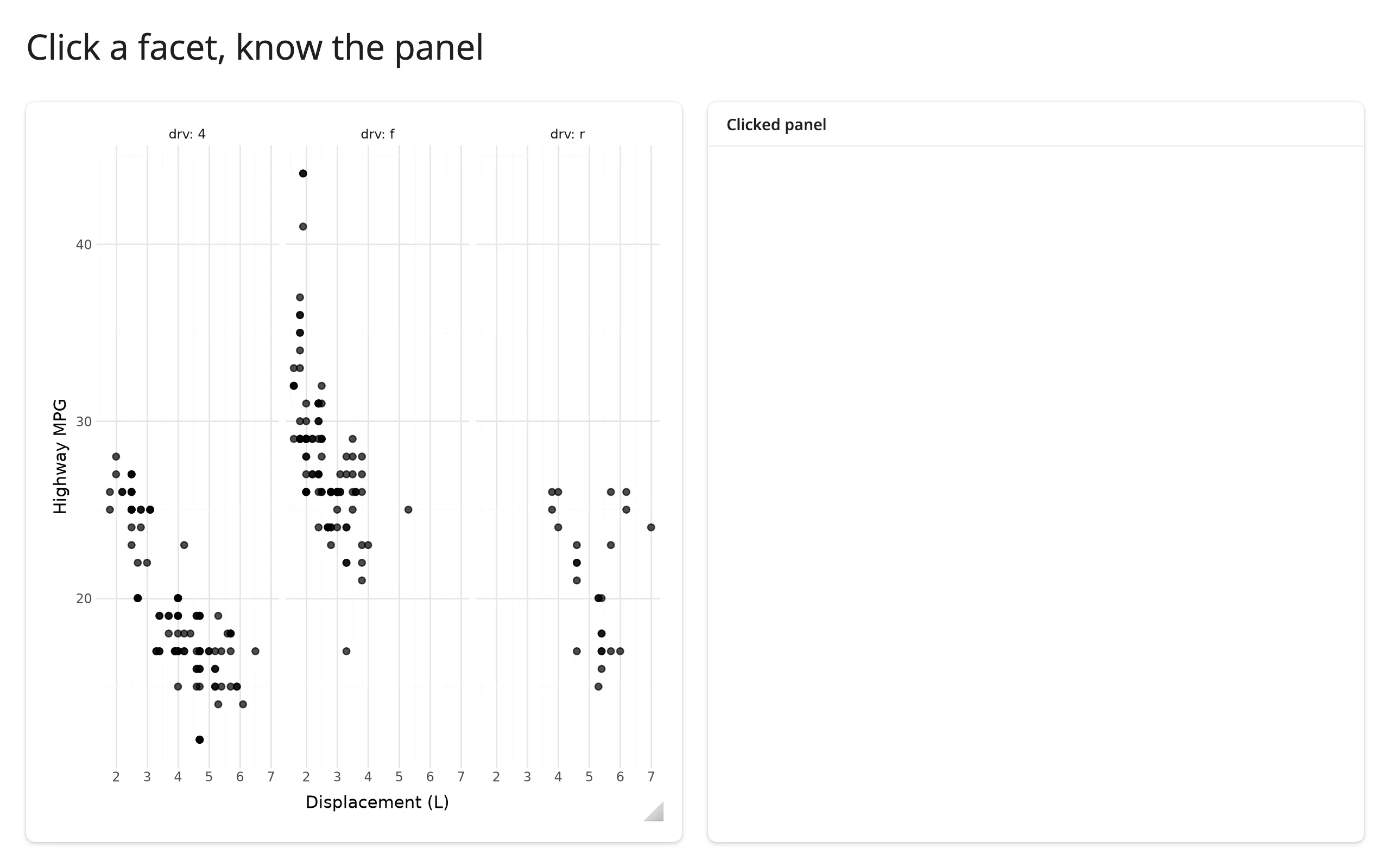
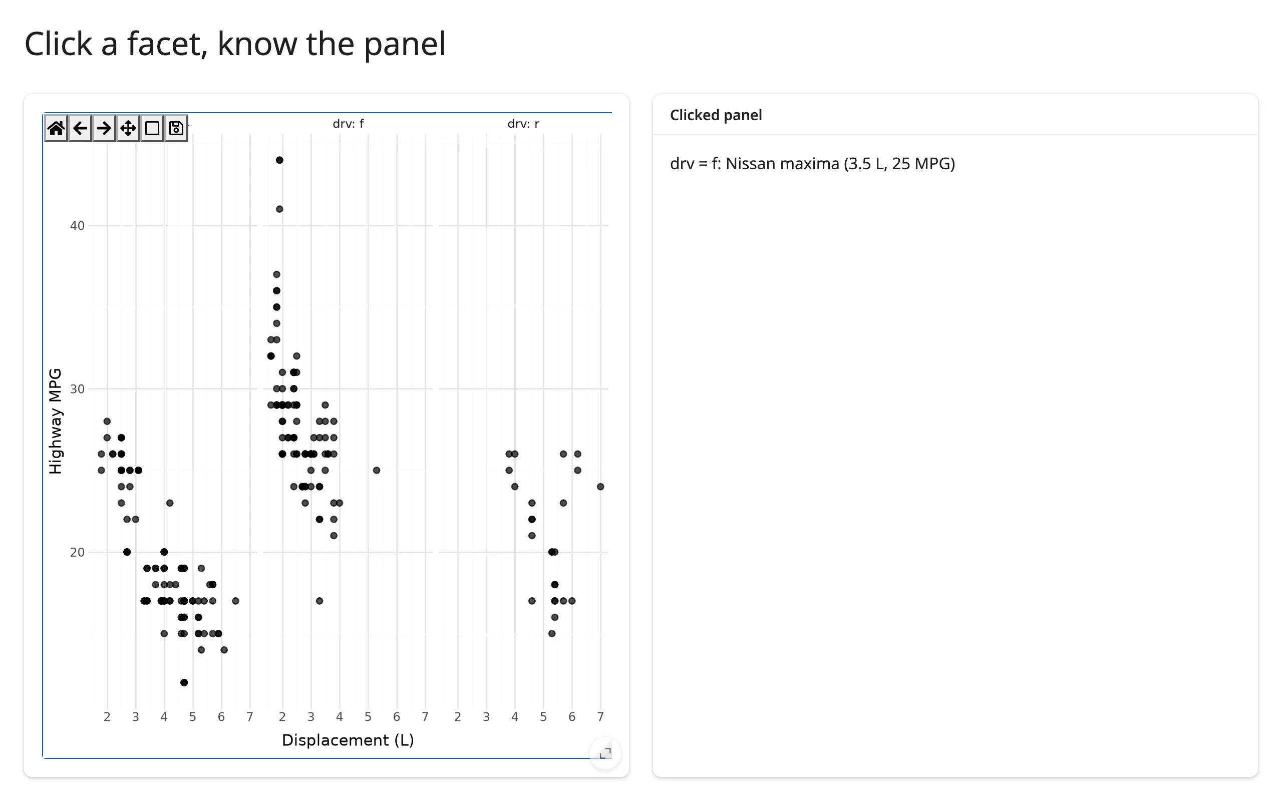
event.inaxes names which Axes the press landed on, but nothing in the event itself names that axes’ facet value – facets are just a grid of ordinary matplotlib axes to the event system. The fix uses one piece of plotnine internals: figure.get_layout_engine().plot is the actual drawn ggplot plotnine attaches to the figure, and its .facet.layout.layout is the data frame that assigns each facet a PANEL number in the same order as figure.axes. figure.axes.index(event.inaxes) gives you the row into that table, and from there the facet’s data value (here, drv). This relies on an undocumented plotnine attribute path (_mpl.layout_manager in the module path), verified against plotnine 0.15.9 – treat it as something to re-check against a plotnine upgrade, not a stable public API.
Zoom drives a second, independently-scaled plot
import matplotlib.dates as mdates
import pandas as pd
from plotnine import aes, geom_line, ggplot, labs, theme_minimal
from plotnine.data import economics
from shiny.express import render, ui
from shinywidgets import render_plotnine

ui.page_opts(title="Zoom drives a linked plot", fillable=True)


def visible_window():
    (x0, x1), _ = top.limits()
    lo = pd.Timestamp(mdates.num2date(x0).replace(tzinfo=None))
    hi = pd.Timestamp(mdates.num2date(x1).replace(tzinfo=None))
    return economics[(economics.date >= lo) & (economics.date <= hi)]


with ui.layout_columns():
    with ui.card(full_screen=True):
        ui.card_header("Unemployment -- zoom into a stretch")

        @render_plotnine
        def top():
            return (
                ggplot(economics, aes("date", "unemploy"))
                + geom_line()
                + labs(x="", y="Unemployed (thousands)")
                + theme_minimal()
            )

    with ui.card(full_screen=True):
        ui.card_header("Savings rate, same window")

        @render_plotnine
        def bottom():
            return (
                ggplot(visible_window(), aes("date", "psavert"))
                + geom_line(color="darkorange")
                + labs(x="", y="Personal savings rate (%)")
                + theme_minimal()
            )


with ui.card():
    ui.card_header("Summary of the visible window")

    @render.text
    def summary():
        visible = visible_window()
        return f"{len(visible)} months visible, average unemployment {visible.unemploy.mean():,.0f}k"
Before zooming, and after box-zooming the top plot into 1978-1991:
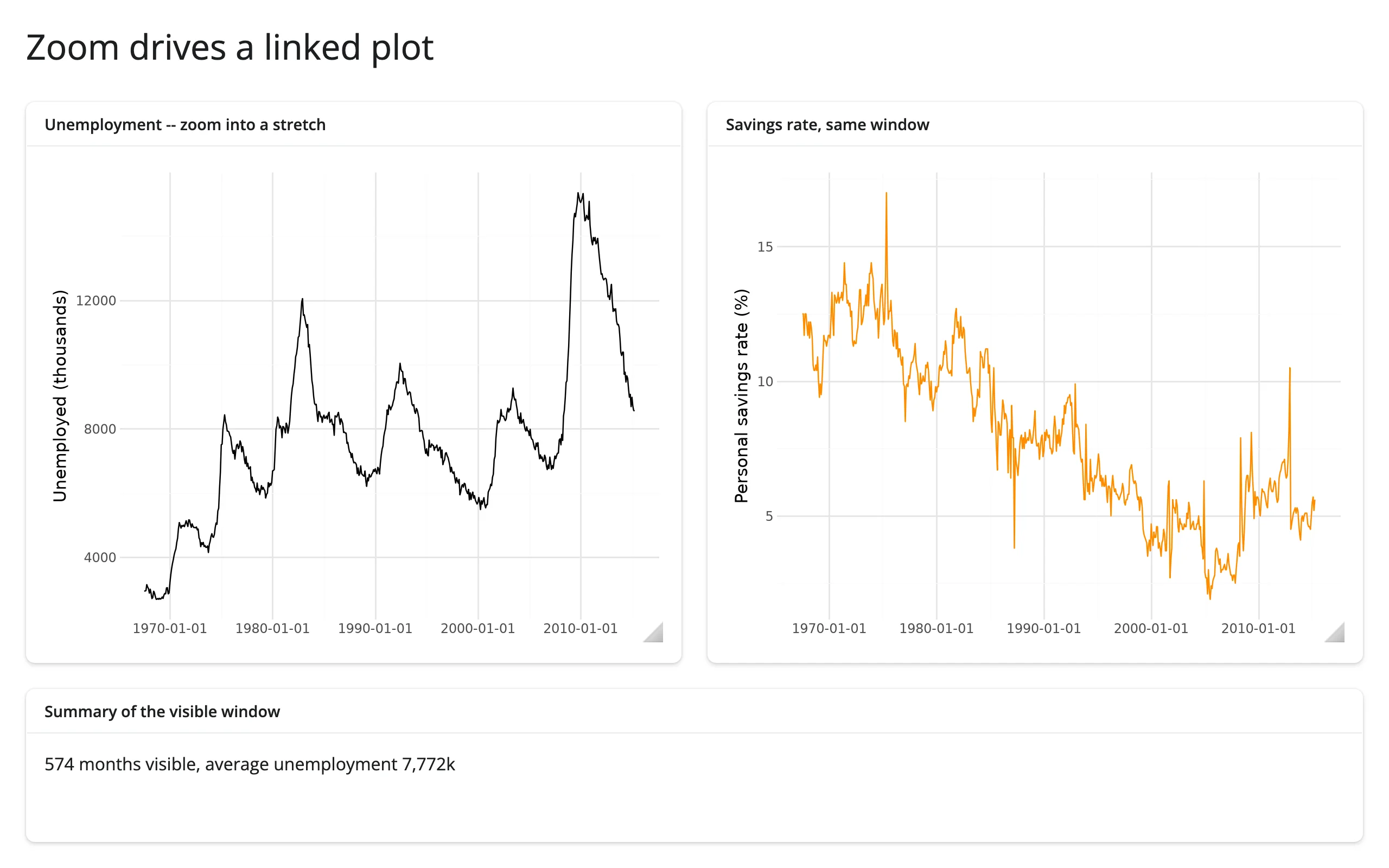
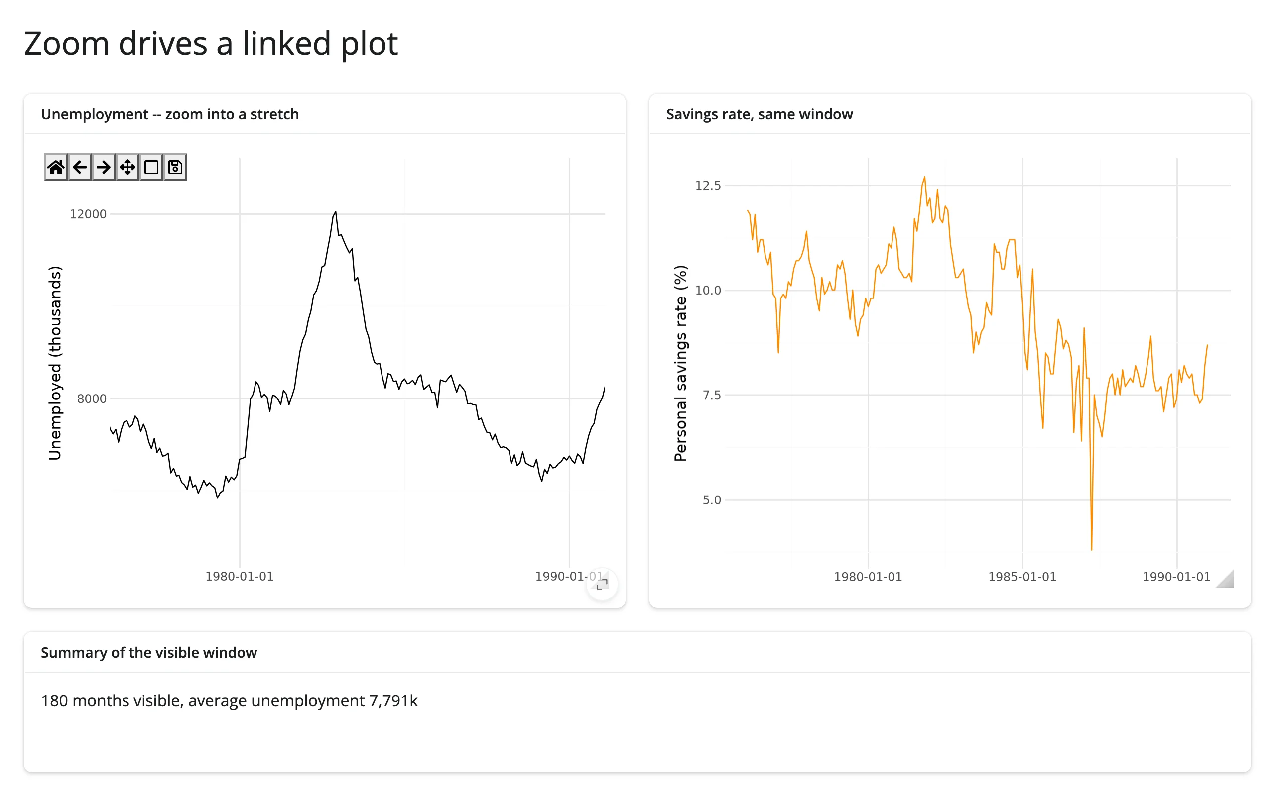
The bottom plot and the summary text both call top.limits() directly – no reactive.value, no ax.callbacks.connect, no separate tracking effect. This is the simplification limits() buys over the hand-rolled recipe earlier versions of this guide taught: reading an accessor from a sibling output is just a function call, and Shiny’s normal reactive graph (bottom/summary depend on top.limits(), which depends on the user’s zoom) handles the rest. The two series have unrelated y-scales (thousands of people vs. a percentage), which is exactly when a second plot, not a shared axis, is the right way to link them – plotnine facets share one scale per row/column, which wouldn’t work here.
Large data
plotnine shares matplotlib’s ipympl engine (see the matplotlib guide) and has no large-data mode of its own: no WebGL, no server-side rasterization, and every pan/zoom redraws the whole figure to a bitmap. See “When to use @render.plot instead” in Gotchas and limitations below for when a static image is the better trade, and reach for bokeh, plotly, or datashader when the data itself needs to scale into the millions. This is the gap the “draw it with the GPU” and “summarize on the server” approaches in Large data & performance fill instead.
Layout and sizing
from plotnine import aes, geom_point, ggplot, theme, theme_minimal
from plotnine.data import mpg
from shiny.express import ui
from shinywidgets import render_plotnine

ui.page_opts(fillable=True)


def scatter():
    return ggplot(mpg, aes("displ", "hwy")) + geom_point() + theme_minimal()


with ui.layout_columns():
    with ui.card(full_screen=True):
        ui.card_header("Fills its card (default)")

        @render_plotnine
        def fills():
            return scatter()

    with ui.card():
        ui.card_header("Explicit height: set a matching figure_size")

        @render_plotnine(height="220px")
        def fixed():
            return scatter() + theme(figure_size=(4, 2.2))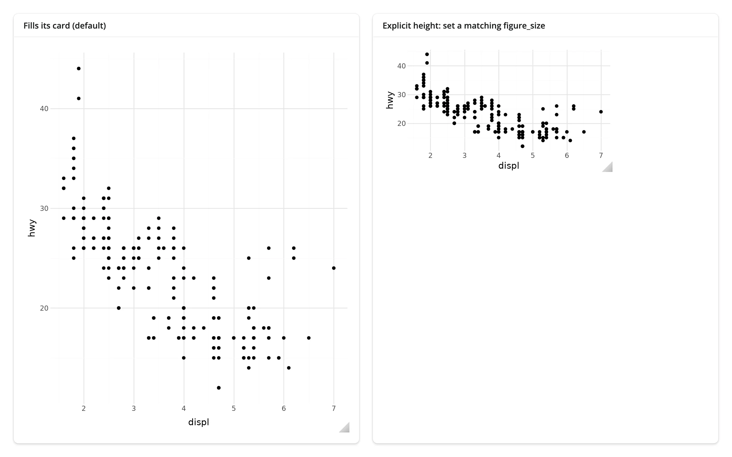
In a filling layout (the default: no height given), render_plotnine resizes the figure to its container on every render and resize, overriding any theme(figure_size=...) you set – that’s the left card above. Give the output an explicit height and the figure is drawn at its figure_size and not fitted to the output: a bigger figure than the output is clipped, so set a matching theme(figure_size=...) yourself, as the right card does. With fill=False and no height, the figure’s width still tracks its container; only the height becomes fixed. Leave theme(dpi=...) at its default (100) in either case – a higher DPI acts like a zoom factor on top of the CSS size rather than a HiDPI setting (HiDPI scaling is automatic: the canvas’s backing store already matches the browser’s device pixel ratio).
You don’t need to hide the canvas chrome yourself: render_plotnine sets canvas.header_visible = False (the “Figure N” label is meaningless once plotnine closes its pyplot figure after drawing – render_matplotlib now defaults to this too) and, unlike render_matplotlib, also canvas.footer_visible = False (the cursor-coordinate readout shows plotnine’s transformed units, e.g., scientific notation under a log scale, which is more confusing than useful).
Gotchas and limitations
Verified on current main (plotnine 0.15.9, shinywidgets main @ 32ca7035, shiny 1.9).
Zooming in close enough can leave an axis with no tick labels at all. plotnine computes its axis breaks once, when it draws (a
FixedLocator/FixedFormatterpair), so a toolbar zoom into a narrow enough window can show only one tick, or none. Verified: zooming a 50-year unemployment series down to a 5-month window left a single “1970-01-01” tick on screen. Fix it in an effect that reads.widget, after the render:import matplotlib.dates as mdates loc = mdates.AutoDateLocator() ax.xaxis.set_major_locator(loc) ax.xaxis.set_major_formatter(mdates.ConciseDateFormatter(loc))For a numeric (non-date) axis, use
matplotlib.ticker.MaxNLocatorandScalarFormatterthe same way. This is an upstream plotnine design choice (interactive zooming isn’t part of its use case), not a shinywidgets bug.Facet panels zoom and pan independently. Each facet is its own matplotlib
Axes; the toolbar’s zoom/pan tools only affect whichever panel the drag started in, even withscales="fixed"(the plotnine default). Link them yourself with matplotlib’sax.sharex()/sharey()if you want zooming one panel to zoom the rest – not verified here in a filling layout, so treat it as a starting point, not a guarantee.Click coordinates are in plotnine’s transformed space, not necessarily your data’s units. Under
scale_x_log10(),event.xdataislog10(x)(confirmed:10 ** event.xdatarecovers the original value, up to axis padding); dates are matplotlib’s ownnum2dateepoch (days since an internal reference date, not your originaldatetime); discrete (categorical) scales use integer positions1..nin the category’s displayed order (confirmed againstggplot(mpg, aes("class", "hwy"))’s 7 classes, positions 1-7).@render.plot’s built-in coordmap converts clicks to data values and facet names for you;render_plotninedoes not, which is the main reason the click-to-row recipes above exist.A plotnine plot has no “update data” API, unlike plotly’s
FigureWidgetor bokeh’sColumnDataSource. In-place updates mean reaching into the matplotlibAxesplotnine drew (see Updating the widget from Python), and the artist index you need (ax.lines[0],ax.collections[0], …) depends on your specific geoms and isn’t part of any stability contract.Returning a non-plot object now raises a clear error. Returning something that isn’t a
ggplotor a composition (e.g.,guide_legend(), which merely has a.draw()method) used to fail deep inside plotnine’s drawing code with a confusingAttributeError. It now raises aTypeErrorup front naming what you returned and what’s expected: “Don’t know how to coerceguide_legend(...)into a plotnine plot: a guide_legend is not a plot. Return a plotnine.ggplot or a plot composition (e.g., p1 | p2).” (verified).req(accessor())can silently swallow a valid falsy result.clicked()itself is immune (aMouseEventis always truthy), but anything you derive from it and store in your ownreactive.value– a row position, an index, a coordinate of0– is not.req(my_value())treats0the same as “nothing yet” and cancels. The accessor examples above all compare toNoneexplicitly for this reason; seeexamples/05_accessor_clicked.py’sdetail()for the pattern. This isn’t specific to plotnine – it applies to any accessor-derived value across the roster – but it’s easy to hit here because “nearest point” naturally produces row position0.When to use
@render.plotinstead: large data (each pan/zoom frame is a fresh server-side Agg render sent as an image – fine for a few thousand points, choppy well before a million), brush-to-select (Shiny’s@render.plot(..., brush=True)ships a rectangular/lasso selection input thatrender_plotninehas no equivalent for), or a dashboard with many small static plots where the ipympl canvas’s per-plot overhead isn’t worth it. Userender_plotninewhen the point is exploration: long time series where the story is in the zoom, scatter plots where clicking a point should explain it, or a composition that needs to be one widget.
Gallery candidates
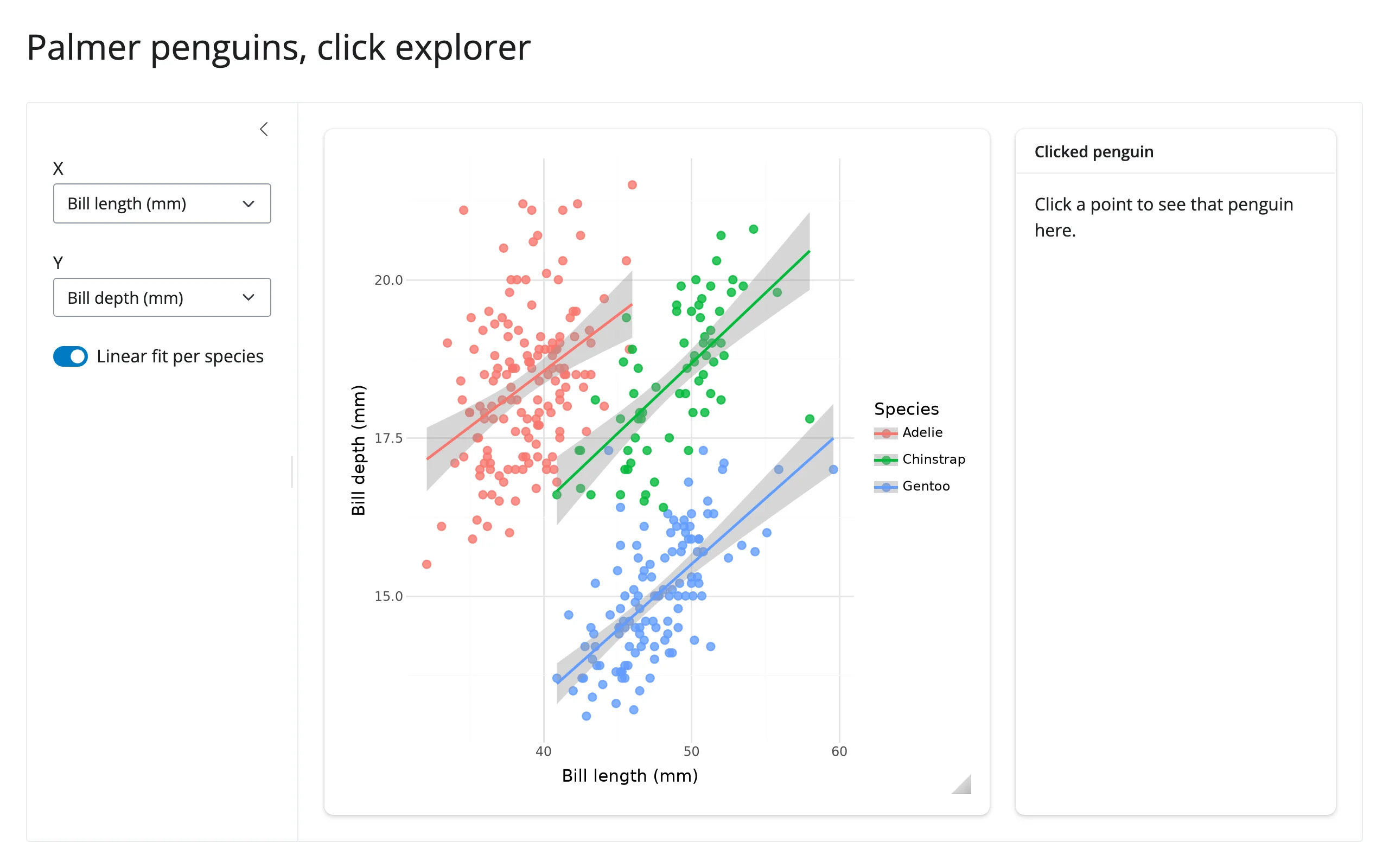
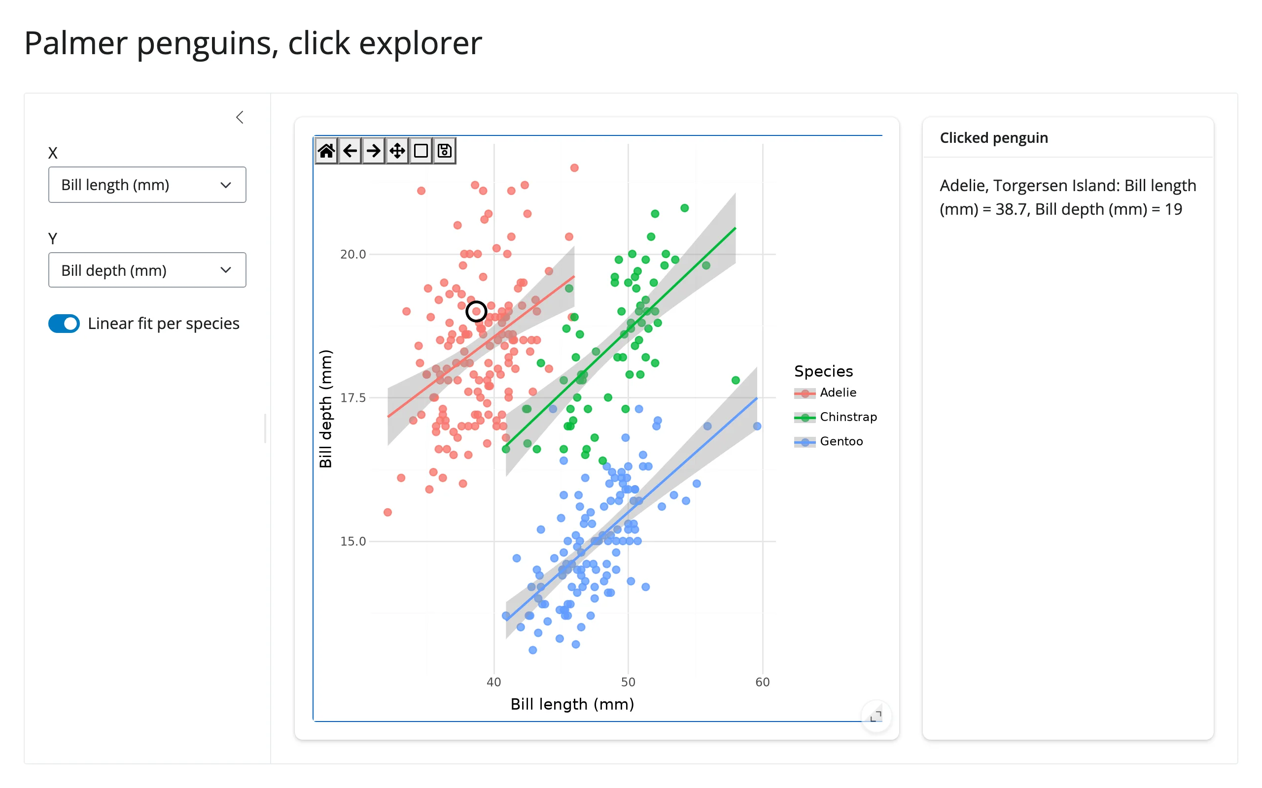
template_click_explorer.py (template) – a Palmer penguins scatter plot with axis pickers and a linear-fit toggle in the sidebar; clicking a point circles it in place and fills in a detail card. Minimal, adaptable starting point for any “explore, then click to inspect” app.
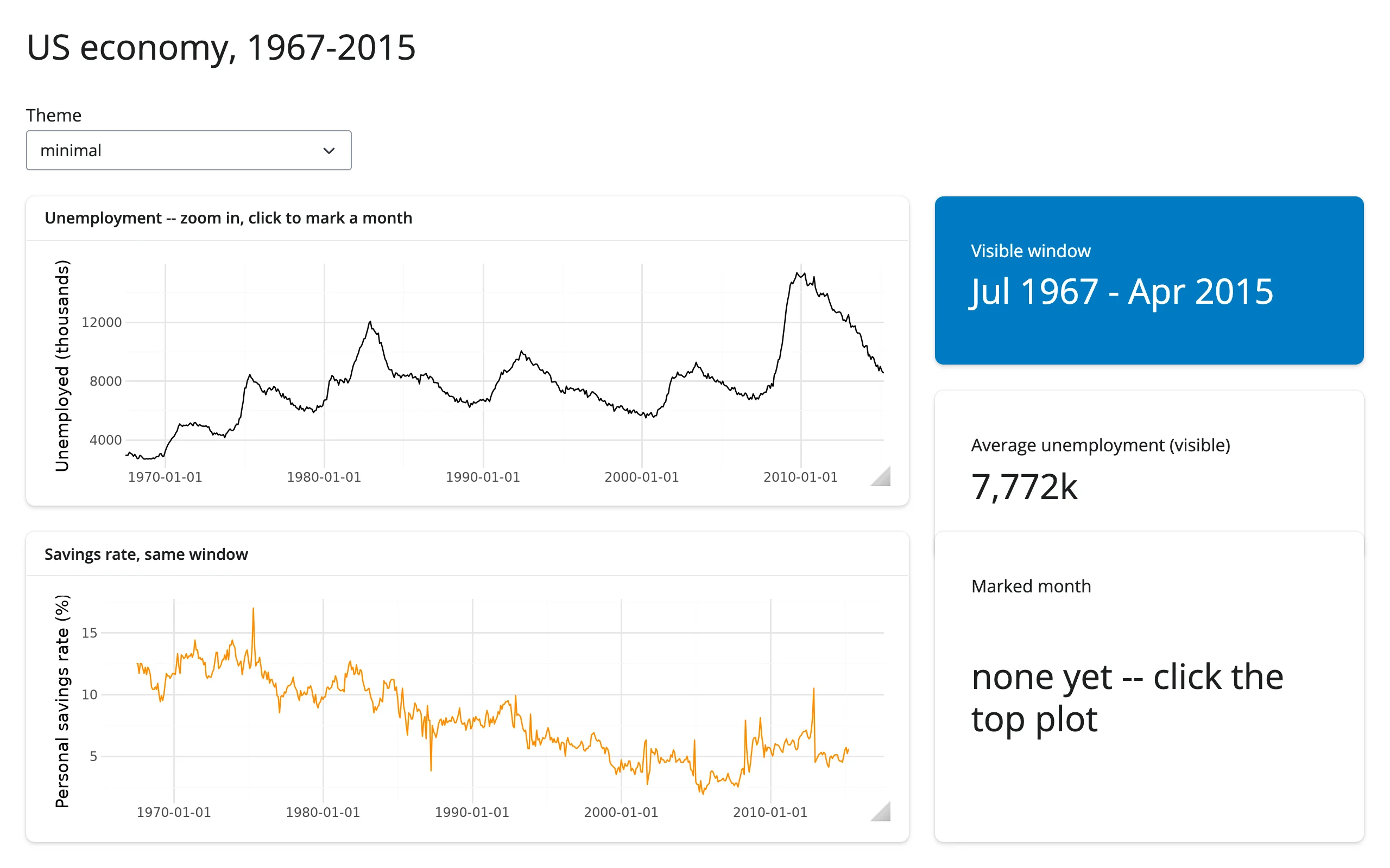
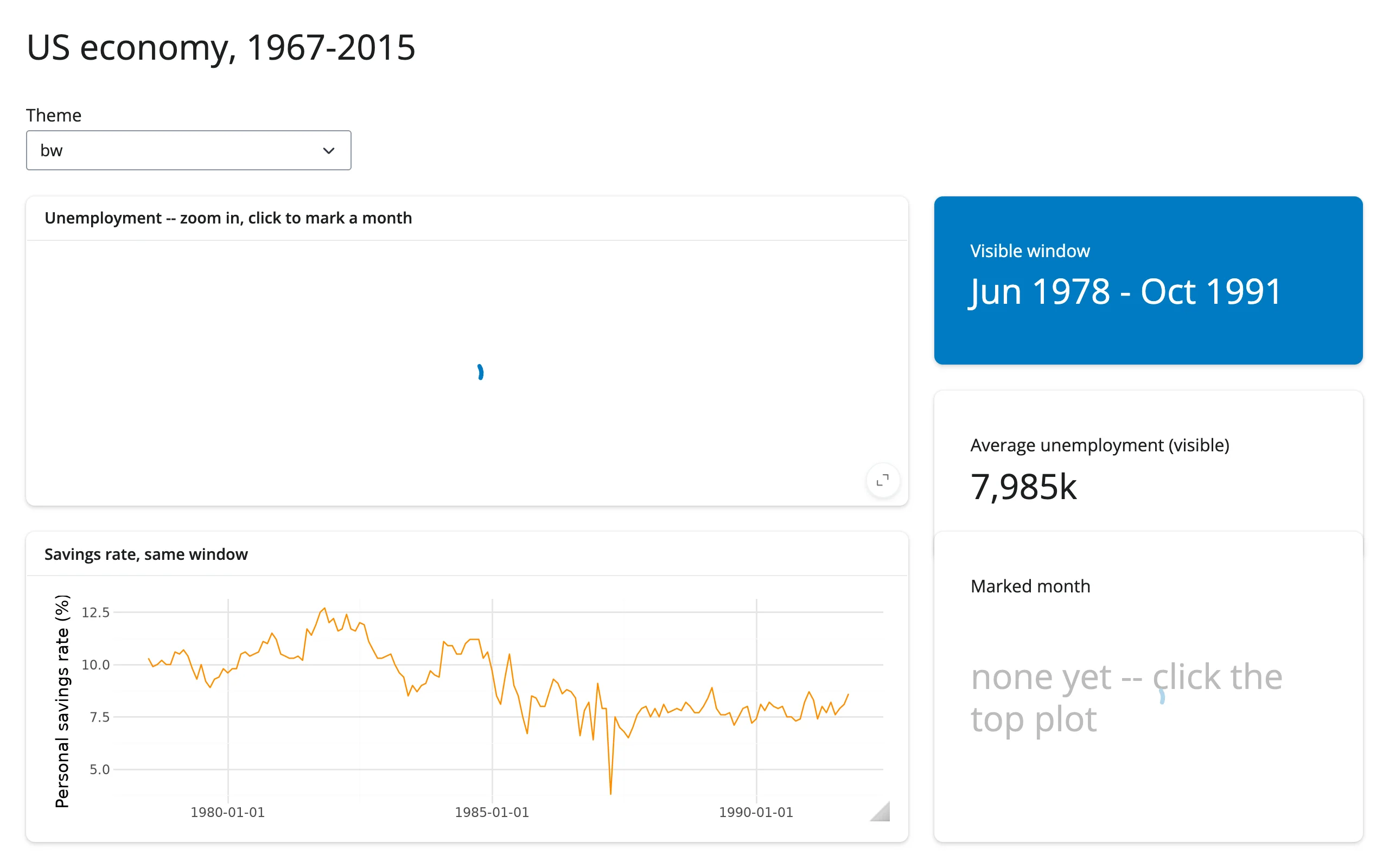
showcase_economics_dashboard.py (showcase) – fifty years of the US economy in one dashboard: zoom the unemployment series and a linked savings-rate plot and a value box follow the visible window (limits()); click to mark a month with an ordinary geom_vline() layer (the click effect feeds the month back into the render); switch the plotnine theme and both the zoom and the mark survive the re-render (the zoom re-applied from an effect that reads .widget, the same technique as Updating the widget from Python).
Learn more
- plotnine documentation – the full geom/scale/theme/facet reference and gallery.
- plotnine’s composition guide – the
|//operators used above, plusplot_spacer()and sizing controls for compositions. - matplotlib guide – the shared ipympl canvas,
clicked()/picked()/limits(), and the general in-place-update technique this guide builds on. - render.plot (Shiny core docs) – the static alternative, including its built-in click/hover/brush inputs and plotnine-aware coordinate mapping.