ipyvolume

Orbit real 3D point clouds, volumes, and surfaces in a Shiny app, with the camera itself as a reactive input.

ipyvolume is a WebGL-based 3D plotting library for Jupyter, written by Maarten Breddels. It does four things that most Python 3D options don’t: real-time volume rendering of 3D arrays (ray-marched in the browser), GPU-instanced scatter/quiver plots of tens of thousands of points, surface and mesh plotting, and built-in frame-by-frame animation with a client-side Play control. All of it runs on three.js underneath (it shares a camera type with pythreejs).

@render_ipyvolume accepts anything that produces an ipyvolume.Figure: the classic pylab API (ipv.figure() / ipv.scatter() / ipv.quickscatter(), returning ipv.gcf()), or direct construction (ipyvolume.Figure() with ipyvolume.widgets.Scatter and friends assigned to fig.scatters). The renderer resizes the figure’s WebGL canvas to fill its container (tracking resizes) unless you give it an explicit size, and it exposes one reactive accessor, camera(), which turns every mouse-drag orbit into a value any other output can read – the camera becomes a first-class reactive input, the same way input.my_slider() is.

Reach for ipyvolume when you need genuine volumetric rendering or a GPU-friendly 3D point cloud/quiver/mesh and don’t need the broader scene-graph control of pythreejs or the picking/physics of pyvista. It’s the only option in the roster for ray-marched volume rendering of a 3D array. If you need object picking, per-vertex selection that maps back to data indices, or very large point clouds (100k+), see k3d or pythreejs instead (this guide’s Gotchas section is specific about where ipyvolume falls short).

hero

One thing to know up front: ipyvolume has had no release since 0.6.3 (2021) and its upstream repo is largely dormant. It still works well for the things this guide covers, but don’t expect upstream fixes – treat the Gotchas section below as load-bearing, not optional reading.

Installation

pip install 'shinywidgets[ipyvolume]'

ipyvolume 0.6.3 imports ipython_genutils but doesn’t declare it as a dependency; the ipyvolume extra installs it for you. Requires ipywidgets 8.1+.

Quick start

The pylab API is the fastest way to get a figure on screen: draw with ipv.quickscatter() (or ipv.scatter()/ipv.figure()), then return the current figure (examples/01_quickstart.py, plotting the bundled iris dataset in 3D):

examples/01_quickstart.py28 lines

import ipyvolume as ipv
import numpy as np
import plotly.express as px
from shiny.express import ui

from shinywidgets import render_ipyvolume

iris = px.data.iris()
# Per-point color must be a numeric (N, 3) RGB array in [0, 1] -- a per-point
# array of color *strings* (e.g. "tomato") hangs ipyvolume's serializer; see
# the "Gotchas" section.
palette = np.array([[0.91, 0.30, 0.24], [0.18, 0.49, 0.20], [0.21, 0.45, 0.69]])
color = palette[iris["species_id"] - 1]

ui.page_opts(title="ipyvolume quickstart", fillable=True)


@render_ipyvolume
def plot():
    ipv.quickscatter(
        iris["sepal_length"],
        iris["petal_length"],
        iris["sepal_width"],
        size=1.2,
        marker="sphere",
        color=color,
    )
    return ipv.gcf()

The runnable version below colors by species instead of drawing from a normal distribution, so the result is recognizable at a glance:

examples/01_quickstart.py28 lines

import ipyvolume as ipv
import numpy as np
import plotly.express as px
from shiny.express import ui

from shinywidgets import render_ipyvolume

iris = px.data.iris()
# Per-point color must be a numeric (N, 3) RGB array in [0, 1] -- a per-point
# array of color *strings* (e.g. "tomato") hangs ipyvolume's serializer; see
# the "Gotchas" section.
palette = np.array([[0.91, 0.30, 0.24], [0.18, 0.49, 0.20], [0.21, 0.45, 0.69]])
color = palette[iris["species_id"] - 1]

ui.page_opts(title="ipyvolume quickstart", fillable=True)


@render_ipyvolume
def plot():
    ipv.quickscatter(
        iris["sepal_length"],
        iris["petal_length"],
        iris["sepal_width"],
        size=1.2,
        marker="sphere",
        color=color,
    )
    return ipv.gcf()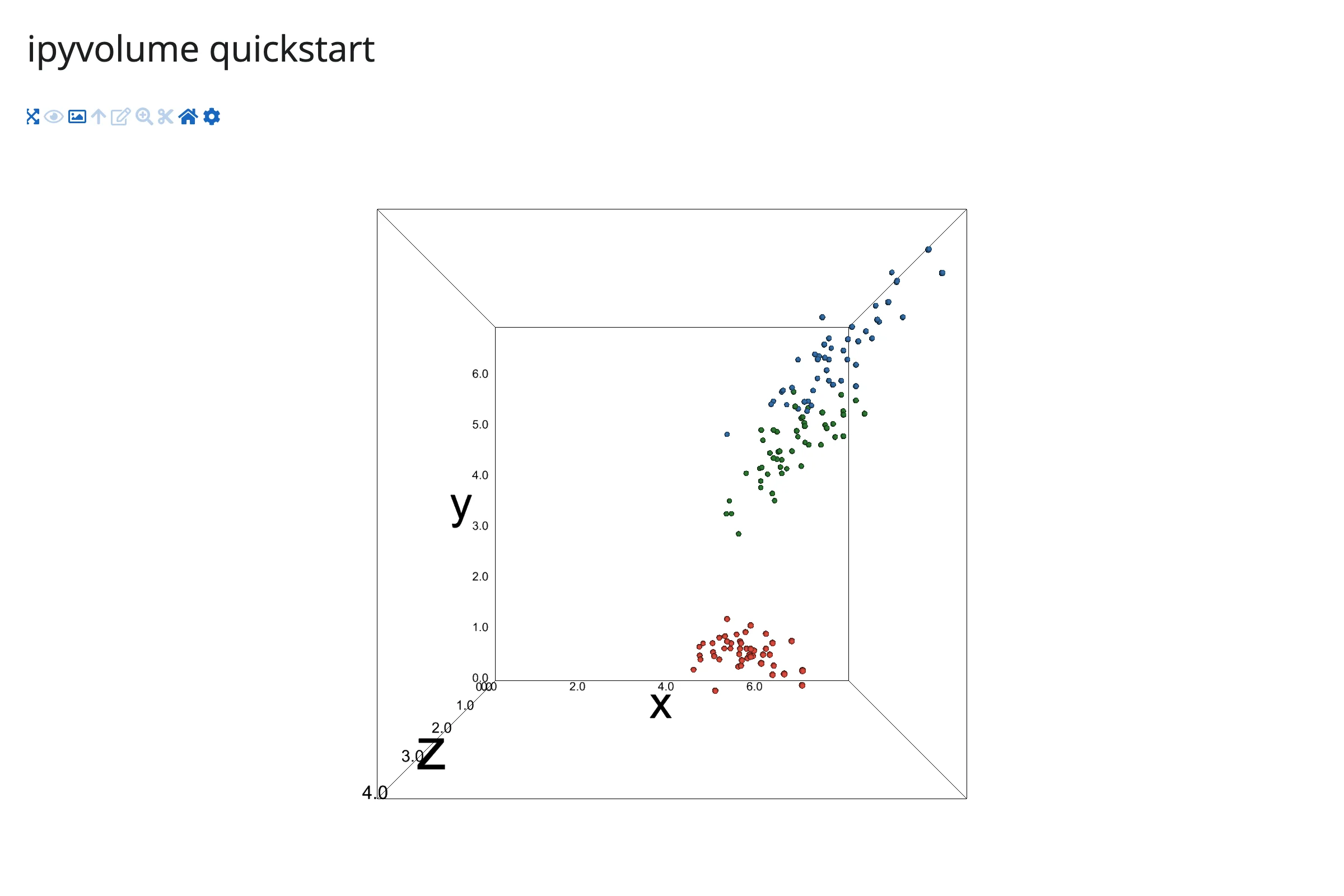

quickstart

What you can build

Volume rendering

ipv.volshow()/ipv.quickvolshow() ray-march a 3D numpy array in the browser – give it a density field (medical imaging, simulation output, a 3D histogram) and it renders translucent iso-surfaces at the levels you choose, with no VTK or server-side rendering involved.

examples/02_volume.py21 lines

import ipyvolume as ipv
import numpy as np
from shiny.express import ui

from shinywidgets import render_ipyvolume

ui.page_opts(title="Volume rendering", fillable=True)

# A synthetic density field (two overlapping Gaussian blobs) standing in for
# a CT/MRI-style 3D array -- any (nx, ny, nz) numpy array works.
grid = np.linspace(-1, 1, 64)
gx, gy, gz = np.meshgrid(grid, grid, grid, indexing="ij")
blob_a = np.exp(-((gx - 0.25) ** 2 + gy**2 + gz**2) / 0.05)
blob_b = np.exp(-((gx + 0.3) ** 2 + (gy - 0.2) ** 2 + gz**2) / 0.08)
density = blob_a + 0.7 * blob_b


@render_ipyvolume
def plot():
    ipv.quickvolshow(density, level=[0.2, 0.5, 0.8], opacity=[0.01, 0.05, 0.12])
    return ipv.gcf()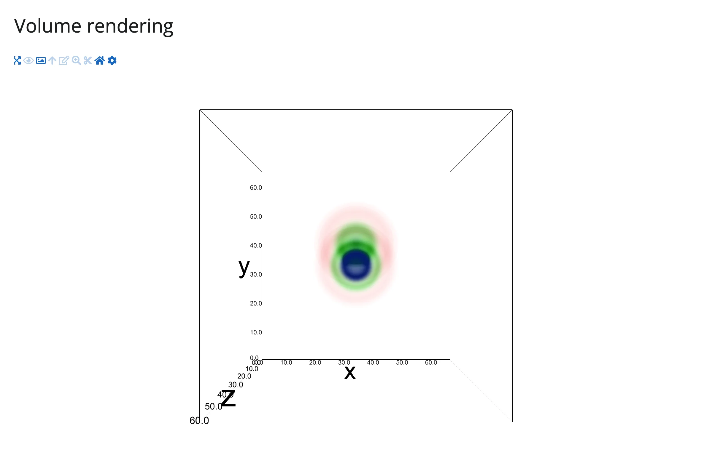

volume

Quiver (vector fields)

ipv.quiver() is a scatter plot with arrows: give it points and (u, v, w) directions and it draws one arrow per point, GPU-instanced like the scatter marker.

examples/03_quiver.py21 lines

import ipyvolume as ipv
import numpy as np
from shiny.express import ui

from shinywidgets import render_ipyvolume

ui.page_opts(title="Quiver", fillable=True)

# A synthetic vortex vector field: points on a grid, with (u, v, w) giving
# the arrow direction at each point.
lin = np.linspace(-2, 2, 6)
x, y, z = np.meshgrid(lin, lin, lin, indexing="ij")
x, y, z = x.ravel(), y.ravel(), z.ravel()
u, v, w = -y, x, np.zeros_like(z) + 0.3


@render_ipyvolume
def plot():
    ipv.figure()
    ipv.quiver(x, y, z, u, v, w, size=8, color="steelblue")
    return ipv.gcf()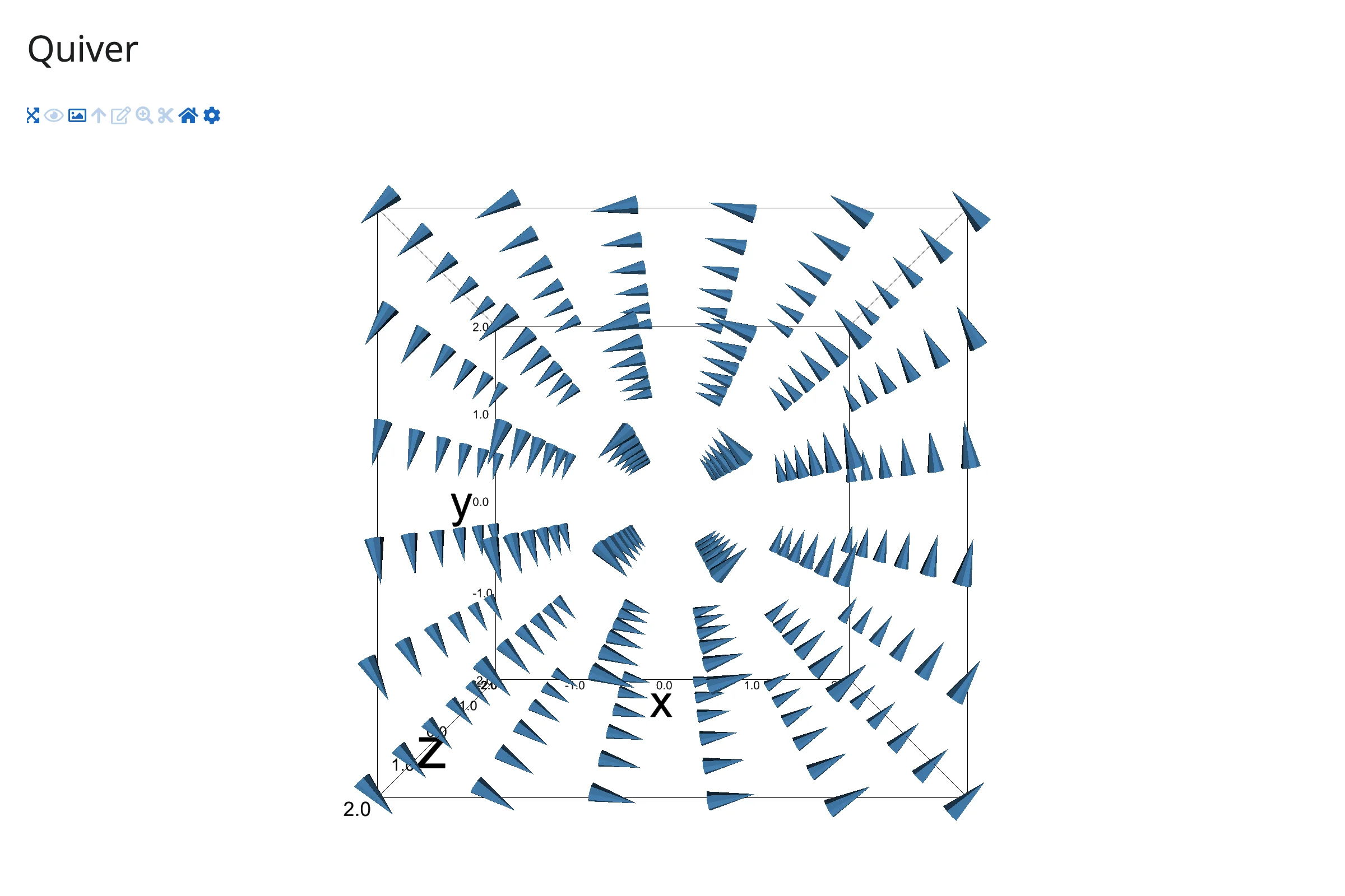

quiver

Surfaces and wireframes

ipv.plot_surface()/ipv.plot_wireframe()/ipv.plot_mesh() take 2D-ordered x, y, z arrays (a mathematical surface, a terrain grid) and auto-fit the axes for you.

examples/04_surface.py20 lines

import ipyvolume as ipv
import numpy as np
from shiny.express import ui

from shinywidgets import render_ipyvolume

ui.page_opts(title="Surface", fillable=True)

u = np.linspace(-5, 5, 60)
x, y = np.meshgrid(u, u)
r = np.sqrt(x**2 + y**2) + 1e-6
z = np.sin(r) / r


@render_ipyvolume
def plot():
    ipv.figure()
    ipv.plot_surface(x, z, y, color="orange")
    ipv.plot_wireframe(x, z, y, color="black")
    return ipv.gcf()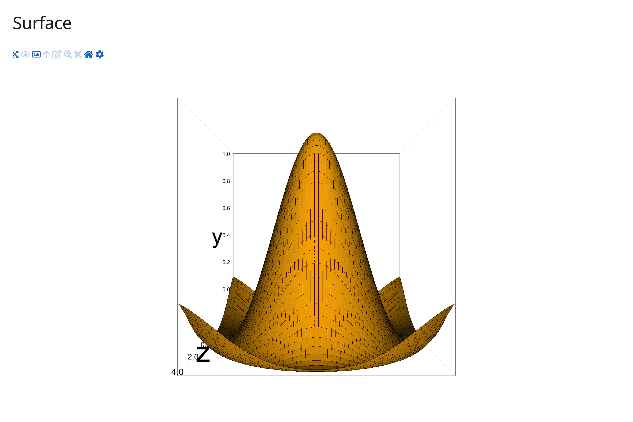

surface

Animation

ipv.animation_control() turns a Scatter whose arrays have an extra leading “frame” axis into an animated comet, with a client-side Play/stop/loop control – no Python callback runs per frame. The control is a separate widget: with add=False it returns the Play/slider HBox for you to render as a second output (the default add=True instead drops it into the pylab container, which isn’t visible if your render function returns the bare Figure).

examples/05_animation.py34 lines

import ipyvolume as ipv
import numpy as np
from shiny.express import ui

from shinywidgets import render_ipyvolume, render_widget

ui.page_opts(title="Animation", fillable=True)

# A helix traced out over time: shape (frames, points, 3). The first axis is
# the animation sequence -- get this axis order wrong and the animation plays
# the wrong dimension.
t = np.linspace(0, 4 * np.pi, 300)
helix = np.stack([np.cos(t), np.sin(t), t / 4], axis=1)
frames = np.stack([np.roll(helix, -i, axis=0)[:40] for i in range(len(t))])


@render_ipyvolume
def plot():
    fig = ipv.figure()
    ipv.scatter(
        frames[:, :, 0], frames[:, :, 1], frames[:, :, 2], size=1.5, marker="sphere", color="steelblue"
    )
    return fig


@render_widget
def controls():
    fig = plot.value  # re-runs once `plot` first renders (None before that)
    if fig is None:
        return None
    # add=False returns the Play/slider HBox; the default add=True instead
    # targets the pylab container (invisible here, since `plot` returns the
    # bare Figure) and returns None.
    return ipv.animation_control(fig.scatters[0], add=False, interval=40)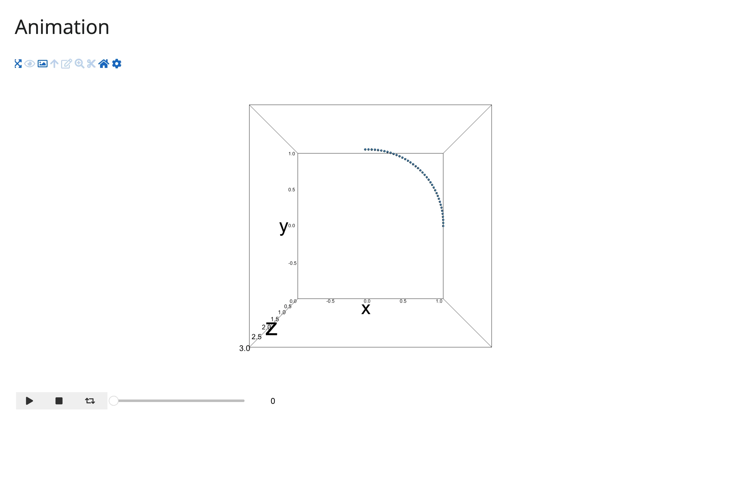

animation

Reacting to user interaction

Accessor reference

Accessor	Returns	Before any interaction	Across re-render	Default rate policy
camera()	the live pythreejs.Camera (same mutable instance every read)	seeded value: the figure’s camera as constructed (never cancels unless fig.camera is explicitly None)	re-seeded to the new figure’s camera	none – the browser already coalesces a whole orbit gesture into one update

camera() fires when the camera’s position/quaternion/zoom change (end of an orbit/zoom) or the camera is replaced.

That’s the only accessor ipyvolume has. There is no selected()/clicked() accessor: selections arrive as raw pixel-region custom messages, not indices (see Gotchas), so there’s nothing index-shaped to expose.

camera()

Orbit the figure and read the live position back in Python – the camera becomes a reactive input, exactly like a slider.

examples/06_camera_accessor.py26 lines

import ipyvolume as ipv
import numpy as np
from shiny.express import render, ui

from shinywidgets import render_ipyvolume

ui.page_opts(title="camera() accessor", fillable=True)

ui.markdown("Drag to orbit the scatter; the camera's live position updates below.")


@render_ipyvolume
def plot():
    rng = np.random.default_rng(0)
    x, y, z = rng.normal(size=(3, 300))
    fig = ipv.figure()
    ipv.scatter(x, y, z, size=1, marker="sphere", color="tomato")
    return fig


@render.code
def camera_position():
    # Fires once per completed orbit; the same live pythreejs.Camera instance
    # is returned every time, so read what you need rather than storing it.
    cam = plot.camera()
    return f"position = ({cam.position[0]:.2f}, {cam.position[1]:.2f}, {cam.position[2]:.2f})"

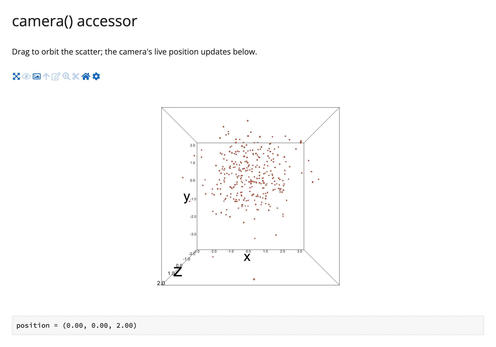
Before the orbit, the camera is still at its construction-time default:

camera before

After a single drag, camera() has fired once with the new position:

camera after

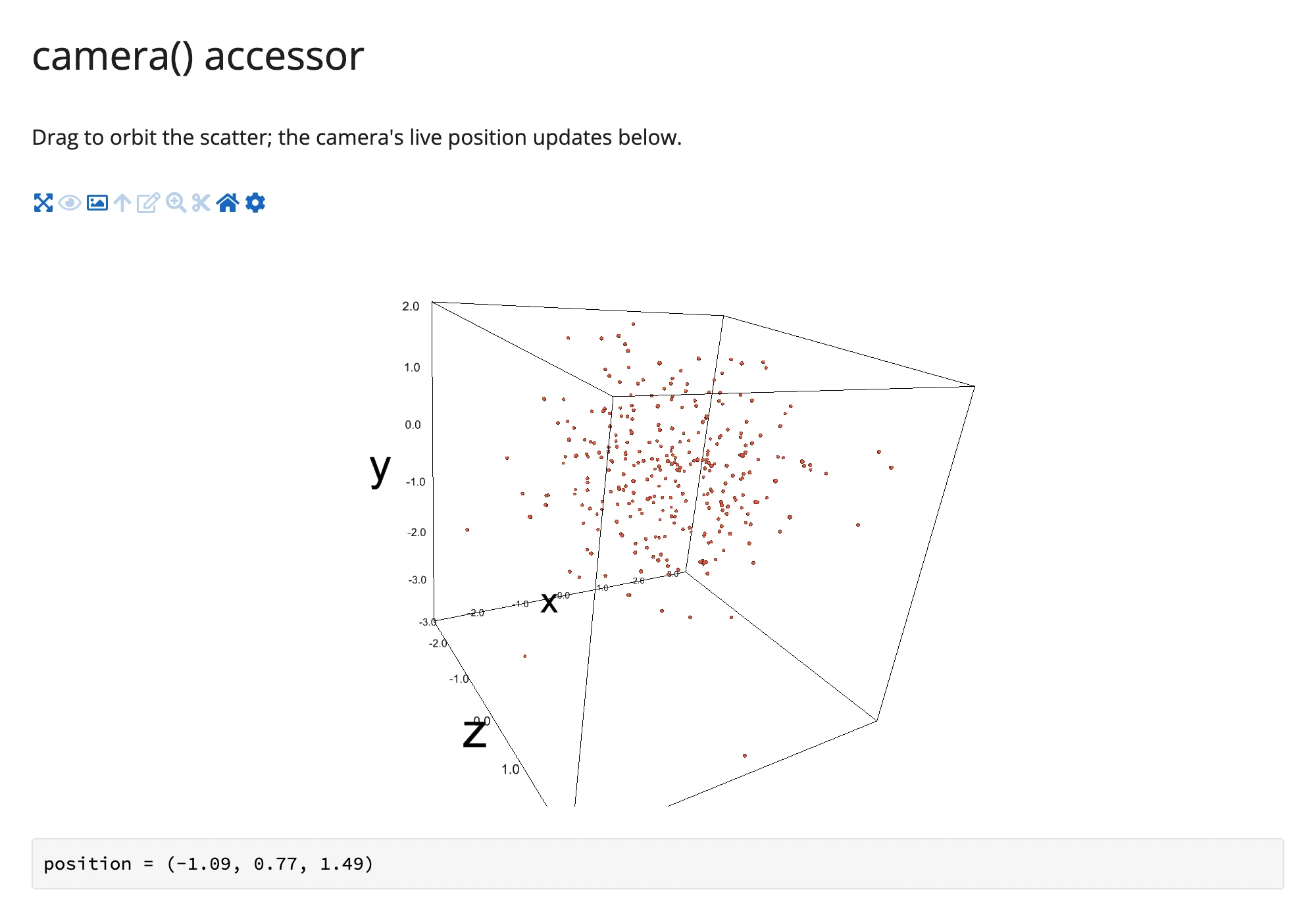
Verified on current main: camera() doesn’t wait for an orbit to return something – read it with no prior interaction and it reports the figure’s camera as constructed (position = (0.00, 0.00, 2.00) for the pylab default above), the same way pythreejs’s camera() does. It only cancels (like req(False)) in the narrow case where fig.camera is explicitly set to None, which the pylab API never does on its own. Across a re-render it re-seeds to the new figure’s camera rather than keeping the old orbit (verified: re-rendering after an orbit drops the camera back to the construction-time default, not the orbited position) – it’s inherent widget state, describing the camera that exists right now, not a one-off interaction to carry over to a figure that no longer exists. (plot.read("camera") is not a substitute for plot.camera(): it returns the raw synced snapshot, not the live Camera object – use the named method.)

Beyond the accessors: reactive_read

A couple of other synced traits are worth reading directly, since they’re not accessors:

• reactive_read(plot.widget, "width") / "height" – the figure’s canvas size in pixels. In a filling layout, the browser measures and resizes the canvas, then syncs the measured size back to these traits; reading them tells you the actual rendered size.
• reactive_read(scatter, "sequence_index") – the current animation frame, if that scatter has an extra frame axis and an animation_control(). This is what lets a companion output track the Play button (see Coordinating multiple views below).

examples/07_reactive_read_beyond.py40 lines

import ipyvolume as ipv
import numpy as np
from shiny.express import render, ui

from shinywidgets import reactive_read, render_ipyvolume, render_widget

ui.page_opts(title="Beyond the accessors", fillable=True)

t = np.linspace(0, 4 * np.pi, 300)
helix = np.stack([np.cos(t), np.sin(t), t / 4], axis=1)
frames = np.stack([np.roll(helix, -i, axis=0)[:40] for i in range(len(t))])

with ui.card(height="320px"):

    @render_ipyvolume
    def plot():
        fig = ipv.figure()
        ipv.scatter(
            frames[:, :, 0], frames[:, :, 1], frames[:, :, 2], size=1.5, marker="sphere", color="steelblue"
        )
        return fig


@render_widget
def controls():
    fig = plot.value
    if fig is None:
        return None
    return ipv.animation_control(fig.scatters[0], add=False, interval=40)


@render.code
def state():
    # The browser syncs the figure's resized canvas back to these traits, and
    # the Play control advances this trait as it animates -- neither is an
    # accessor (no dedicated method), but both are ordinary synced traits.
    w = reactive_read(plot.widget, "width")
    h = reactive_read(plot.widget, "height")
    frame = reactive_read(plot.widget.scatters[0], "sequence_index")
    return f"canvas = {w}x{h}px\nframe = {frame}"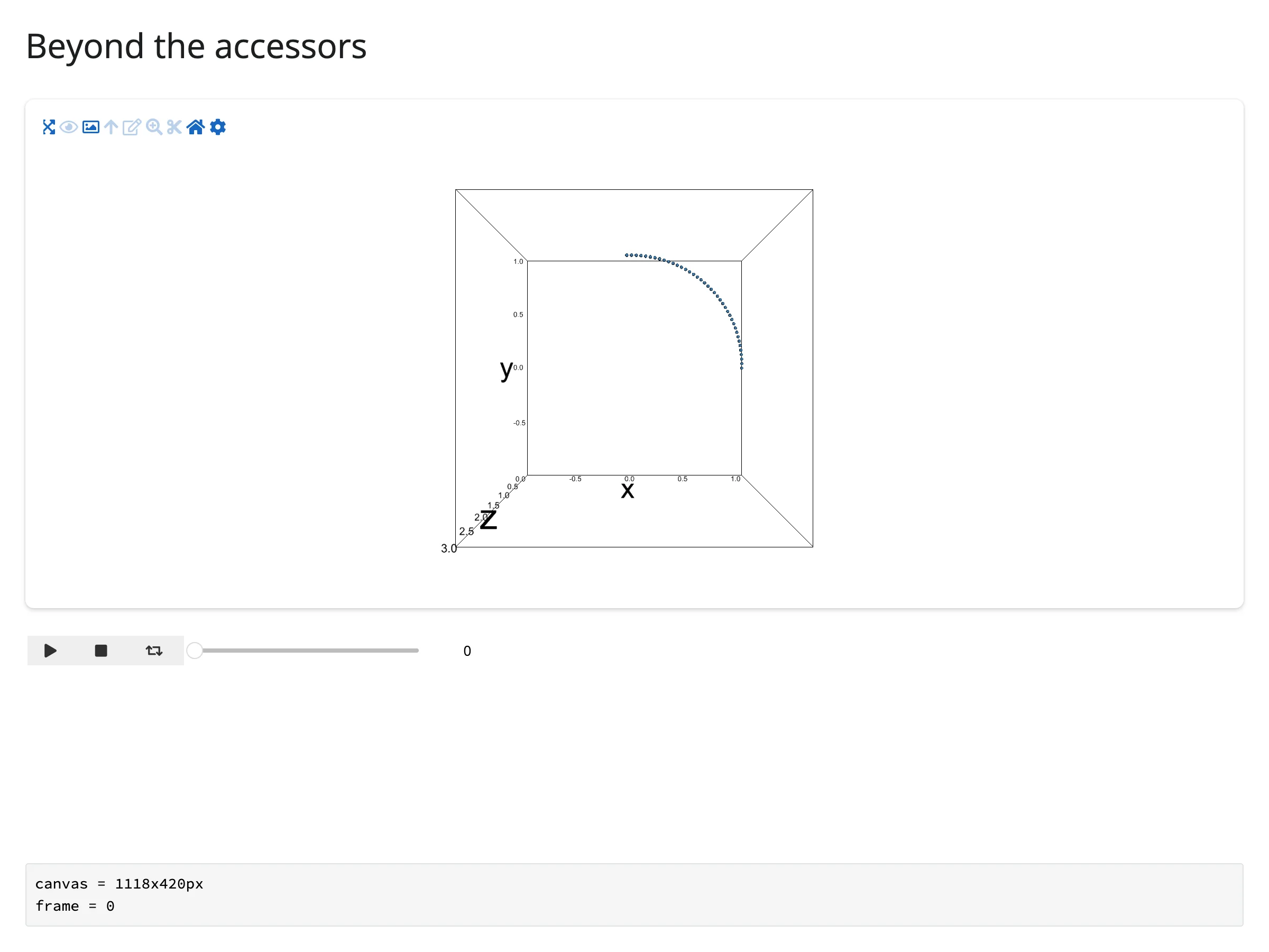

reactive_read

A trait not worth reading this way: scatter.selected. It’s a real synced trait, but it only flows Python-to-browser (see Gotchas) – reactive_read() on it will only ever show you what you last set from Python, never what the user lassoed.

Rate limiting

camera() has no default rate policy because the pythreejs controls already collapse an entire orbit drag into a single trait update – there’s nothing bursty to coalesce. rate_policy/rate_delay still work on render_ipyvolume like any renderer, but for this widget they only affect plain reactive_read() calls on the widget, not camera() itself (an accessor only gets a limiter if its spec declares a default, and camera’s doesn’t).

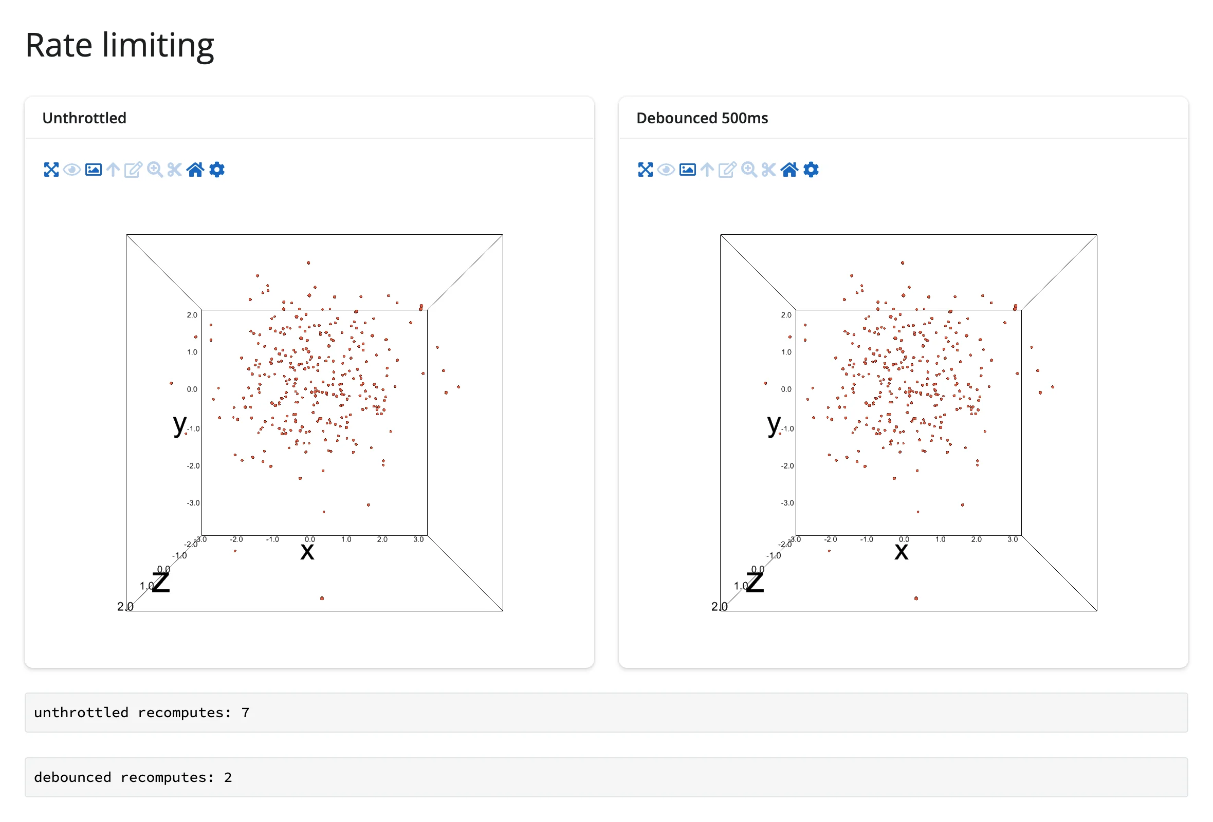
Where that matters in practice: a trait that can update repeatedly, like the canvas size during a container resize. The example below renders two identical figures side by side and counts how often a reactive_read()-driven text output recomputes during a burst of resizes – one unthrottled, one debounced:

examples/08_rate_limiting.py60 lines

import ipyvolume as ipv
import numpy as np
from shiny import reactive
from shiny.express import render, ui

from shinywidgets import reactive_read, render_ipyvolume

# camera() has no default rate policy: a drag already collapses to one trait
# update at the end of the orbit, so there's nothing bursty to coalesce.
# rate_policy/rate_delay still apply to plain reactive_read() calls on the
# widget -- useful for a trait that *does* update repeatedly, like the canvas
# size while its container is being resized.
ui.page_opts(title="Rate limiting", fillable=True)

rng = np.random.default_rng(0)
pts = rng.normal(size=(3, 300))


def make_fig():
    fig = ipv.figure()
    ipv.scatter(*pts, size=1, marker="sphere", color="tomato")
    return fig


with ui.layout_columns():
    with ui.card():
        ui.card_header("Unthrottled")

        @render_ipyvolume
        def plot_live():
            return make_fig()

    with ui.card():
        ui.card_header("Debounced 500ms")

        @render_ipyvolume(rate_policy="debounce", rate_delay=0.5)
        def plot_debounced():
            return make_fig()


live_count = reactive.value(0)
debounced_count = reactive.value(0)


@render.code
def live_recomputes():
    reactive_read(plot_live.widget, "width")
    with reactive.isolate():
        n = live_count.get() + 1
        live_count.set(n)
    return f"unthrottled recomputes: {n}"


@render.code
def debounced_recomputes():
    reactive_read(plot_debounced.widget, "width")
    with reactive.isolate():
        n = debounced_count.get() + 1
        debounced_count.set(n)
    return f"debounced recomputes: {n}"

Mid-burst (7 viewport resizes in quick succession), the unthrottled counter has already advanced with every resize; the debounced one hasn’t moved yet:

rate limiting mid-burst

Updating the widget from Python

Mutating plot.widget in place – rather than re-rendering – keeps the same WebGL canvas and camera, and re-sends only the trait that changed (not the whole point cloud). Use an @reactive.effect for this; wrap reads of your own reactive state in reactive.isolate() if you’d otherwise create a feedback loop.

examples/09_inplace_update.py44 lines

import ipyvolume as ipv
import numpy as np
from shiny import reactive
from shiny.express import input, render, ui

from shinywidgets import render_ipyvolume

# Re-rendering would reset the camera (and re-send all 2,000 points). Mutating
# the already-rendered Scatter's traits in an @reactive.effect instead keeps
# the same WebGL scene -- only the changed trait crosses the wire.
ui.page_opts(title="In-place updates", fillable=True)

ui.input_slider("size", "Point size", 0.2, 3, 1, step=0.1)
ui.input_select("color", "Color", ["tomato", "steelblue", "seagreen"])

rng = np.random.default_rng(0)
pts = rng.normal(size=(3, 2000))


@render_ipyvolume
def plot():
    fig = ipv.figure()
    ipv.scatter(*pts, size=1, marker="sphere", color="tomato")
    return fig


@reactive.effect
def _update_size():
    plot.widget.scatters[0].size = input.size()


@reactive.effect
def _update_color():
    # A single CSS color name is a solid color for every point (cheap, and
    # safe -- see the Gotchas section on *per-point* color arrays).
    plot.widget.scatters[0].color = input.color()


@render.code
def camera_unchanged():
    # Orbit the view, then move the sliders: the camera position you set by
    # dragging is untouched by either effect above.
    cam = plot.camera()
    return f"camera position = ({cam.position[0]:.2f}, {cam.position[1]:.2f}, {cam.position[2]:.2f})"

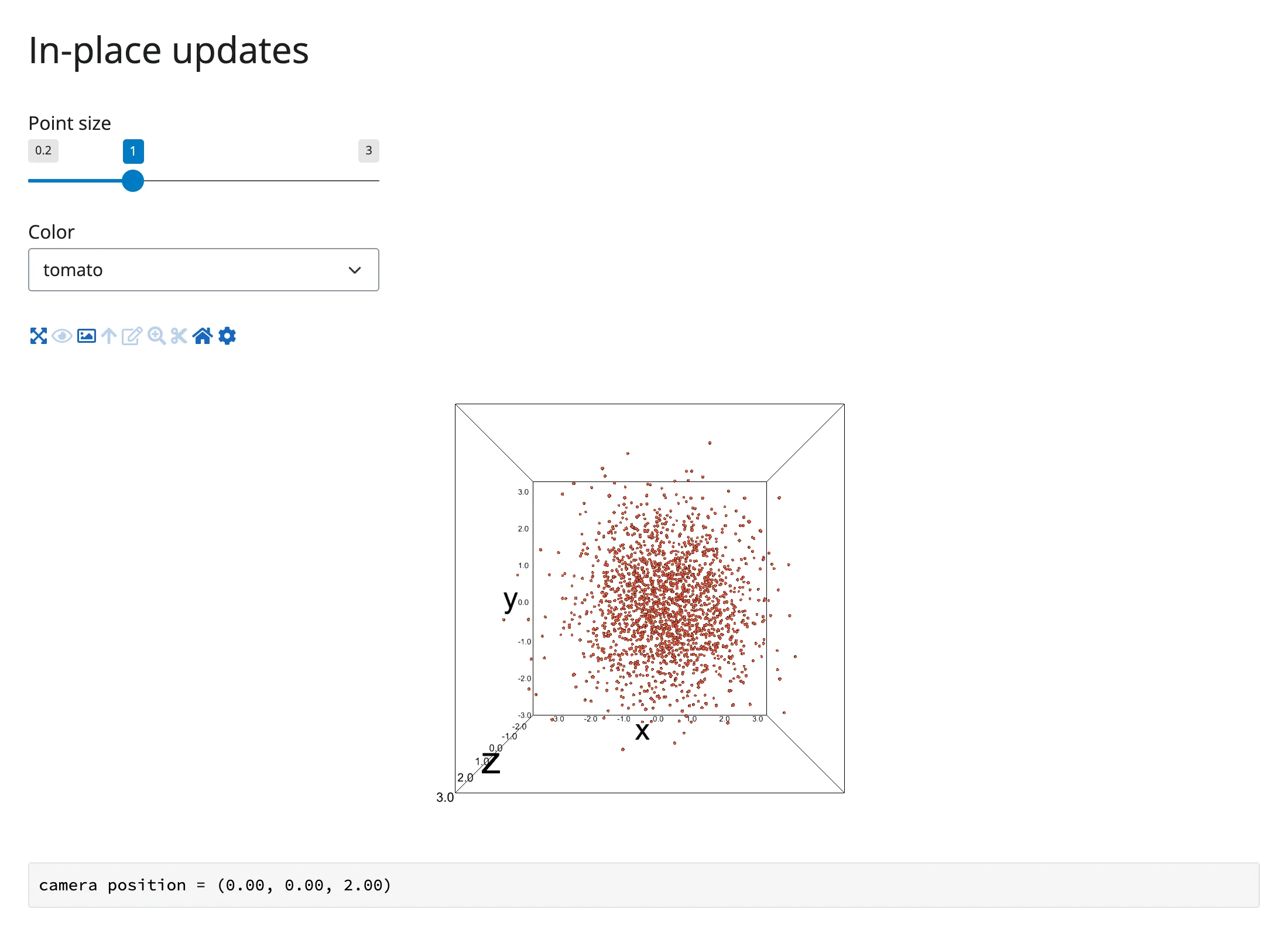
Before: default size and color, camera orbited to a custom position.

in-place before

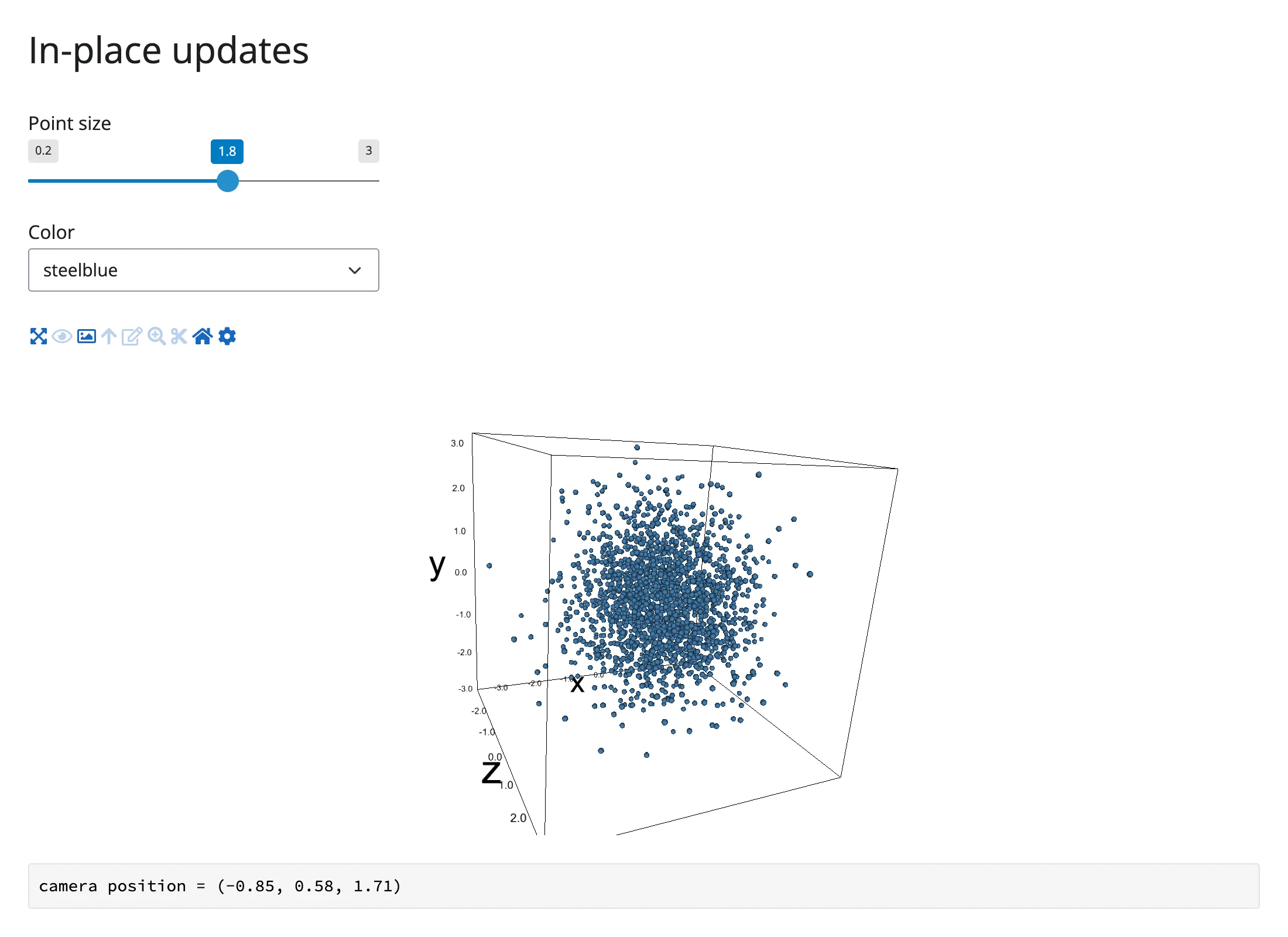
After moving the size slider and switching the color: bigger, blue points, same camera position – confirmed by the readout at the bottom, which matches the value from before.

in-place after

In-place updates beat re-rendering whenever the shape of the data doesn’t change: the browser already has the point cloud, so there’s no reason to re-send it or reset the view. Re-render instead when the dataset itself changes (different x/y/z arrays) or axis limits need to change – direct construction doesn’t auto-fit, so a genuinely new dataset usually needs new xlim/ylim/zlim too.

Coordinating multiple views

Camera-linked twin views

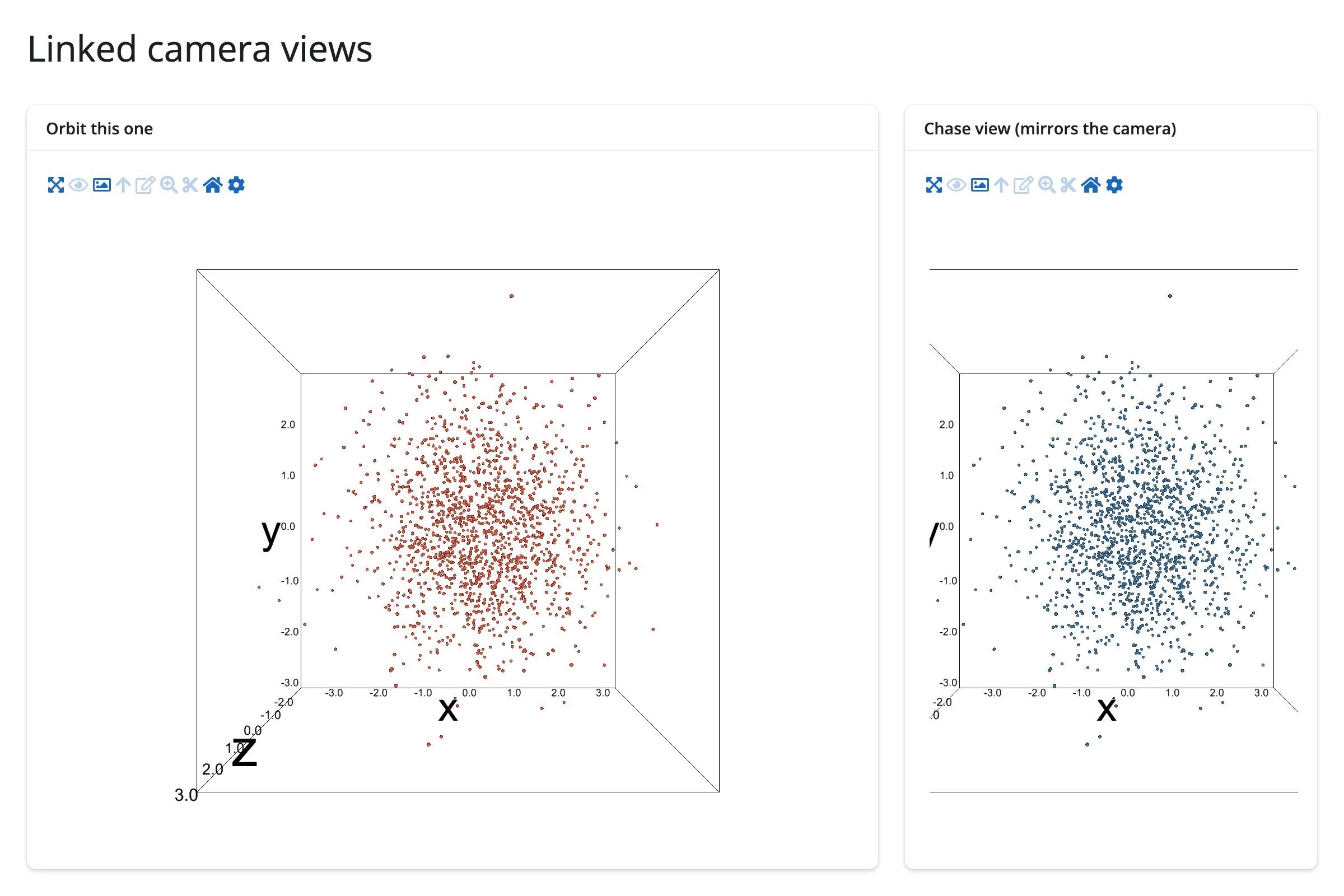
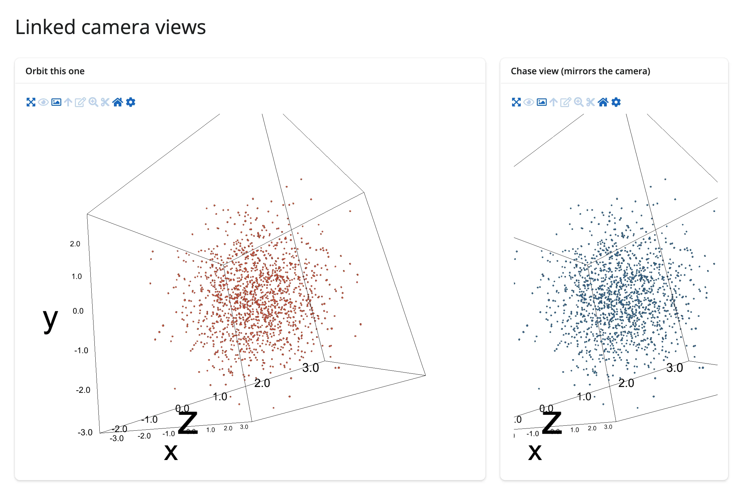
camera() driving another view: orbit one figure, and a second “chase” figure copies the same camera pose. This is the pattern behind an overview/detail pair, or two different representations of the same scene kept in visual sync.

examples/10_linked_camera_views.py41 lines

import ipyvolume as ipv
import numpy as np
from shiny import reactive
from shiny.express import ui

from shinywidgets import render_ipyvolume

# camera() driving another view: orbit the big plot, and a small "chase" view
# mirrors the same camera pose -- a common pattern for a detail/overview pair.
ui.page_opts(title="Linked camera views", fillable=True)

rng = np.random.default_rng(0)
pts = rng.normal(size=(3, 1500))

with ui.layout_columns(col_widths=(8, 4)):
    with ui.card():
        ui.card_header("Orbit this one")

        @render_ipyvolume
        def main_plot():
            fig = ipv.figure()
            ipv.scatter(*pts, size=0.8, marker="sphere", color="tomato")
            return fig

    with ui.card():
        ui.card_header("Chase view (mirrors the camera)")

        @render_ipyvolume
        def chase_plot():
            fig = ipv.figure()
            ipv.scatter(*pts, size=0.8, marker="sphere", color="steelblue")
            return fig


@reactive.effect
def _sync_chase_camera():
    cam = main_plot.camera()
    chase_cam = chase_plot.widget.camera
    chase_cam.position = cam.position
    chase_cam.quaternion = cam.quaternion
    chase_cam.zoom = cam.zoom

Orbiting the left figure moves the right one to match, in the same reactive cycle:

Pairs with: pythreejs (shares the same camera() accessor and Camera type).

Table row selection -> 3D highlight

ipyvolume can’t tell you which points a browser lasso covers (see Gotchas), but nothing stops you driving a highlight the other way: select a row in an ordinary data table and highlight the matching point in 3D. This recomputes plain color/size arrays (baking the highlight into them) rather than using ipyvolume’s dedicated selected/size_selected mechanism – see the Gotchas section for why.

examples/11_table_selection_highlight.py58 lines

import ipyvolume as ipv
import numpy as np
import plotly.express as px
from shiny.express import render, ui

from shinywidgets import render_ipyvolume

# Table row selection -> 3D highlight: ipyvolume can't tell you which points a
# browser lasso covers (see Gotchas), but a table can drive a highlight the
# other way.
#
# This bakes the highlight into plain per-point `color`/`size` arrays rather
# than ipyvolume's dedicated `selected`/`size_selected`/`color_selected`
# mechanism. `selected` has two upstream bugs (see Gotchas): an empty
# `selected=[]` crashes the view, and -- verified separately -- even with a
# non-empty sentinel standing in for "nothing selected", the highlight only
# ever reflects the *first* value `selected` is set to after a figure
# renders; clicking a different row afterwards changes the trait (confirmed
# with `reactive_read`) but never moves the highlighted sphere, with no
# console error. Recomputing a plain color/size array on every selection
# sidesteps both bugs and re-renders the whole figure (the camera resets),
# which is a reasonable trade for a table-driven highlight.
ui.page_opts(title="Table row selection -> 3D highlight", fillable=True)

iris = px.data.iris()
palette = {1: (0.91, 0.30, 0.24), 2: (0.18, 0.49, 0.20), 3: (0.21, 0.45, 0.69)}
base_color = np.array([palette[i] for i in iris["species_id"]])
HIGHLIGHT = np.array([1.0, 1.0, 0.0])  # yellow

with ui.layout_columns():
    with ui.card():
        ui.card_header("Click a row to highlight it in 3D")

        @render.data_frame
        def table():
            return render.DataGrid(
                iris[["sepal_length", "petal_length", "sepal_width", "species"]],
                selection_mode="row",
                height="400px",
            )

    with ui.card():
        ui.card_header("Highlighted point")

        @render_ipyvolume
        def plot():
            rows = list(table.cell_selection()["rows"])
            color = base_color.copy()
            size = np.full(len(iris), 1.2)
            if rows:
                color[rows] = HIGHLIGHT
                size[rows] = 6
            fig = ipv.figure()
            ipv.scatter(
                iris["sepal_length"], iris["petal_length"], iris["sepal_width"],
                size=size, color=color, marker="sphere",
            )
            return fig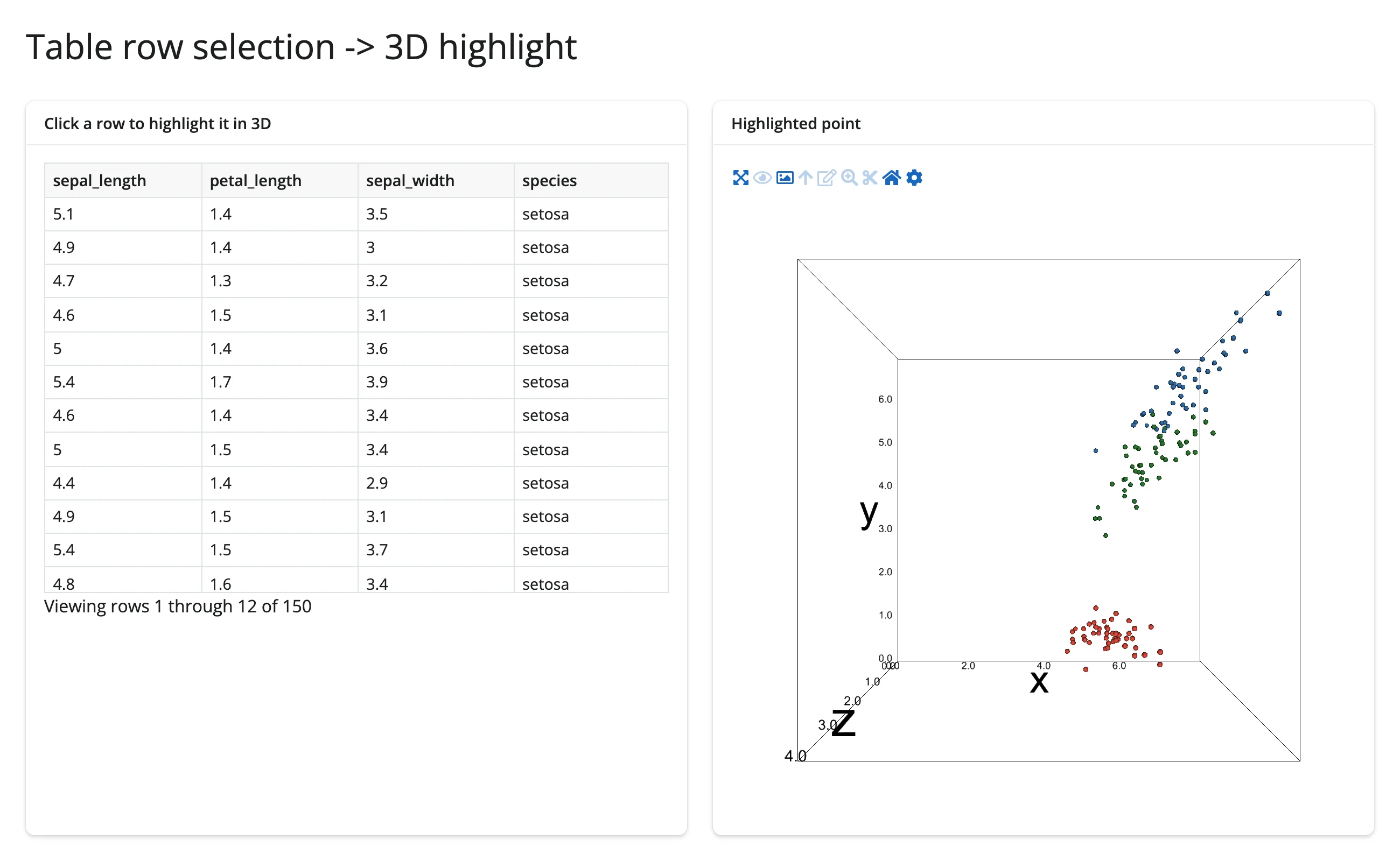

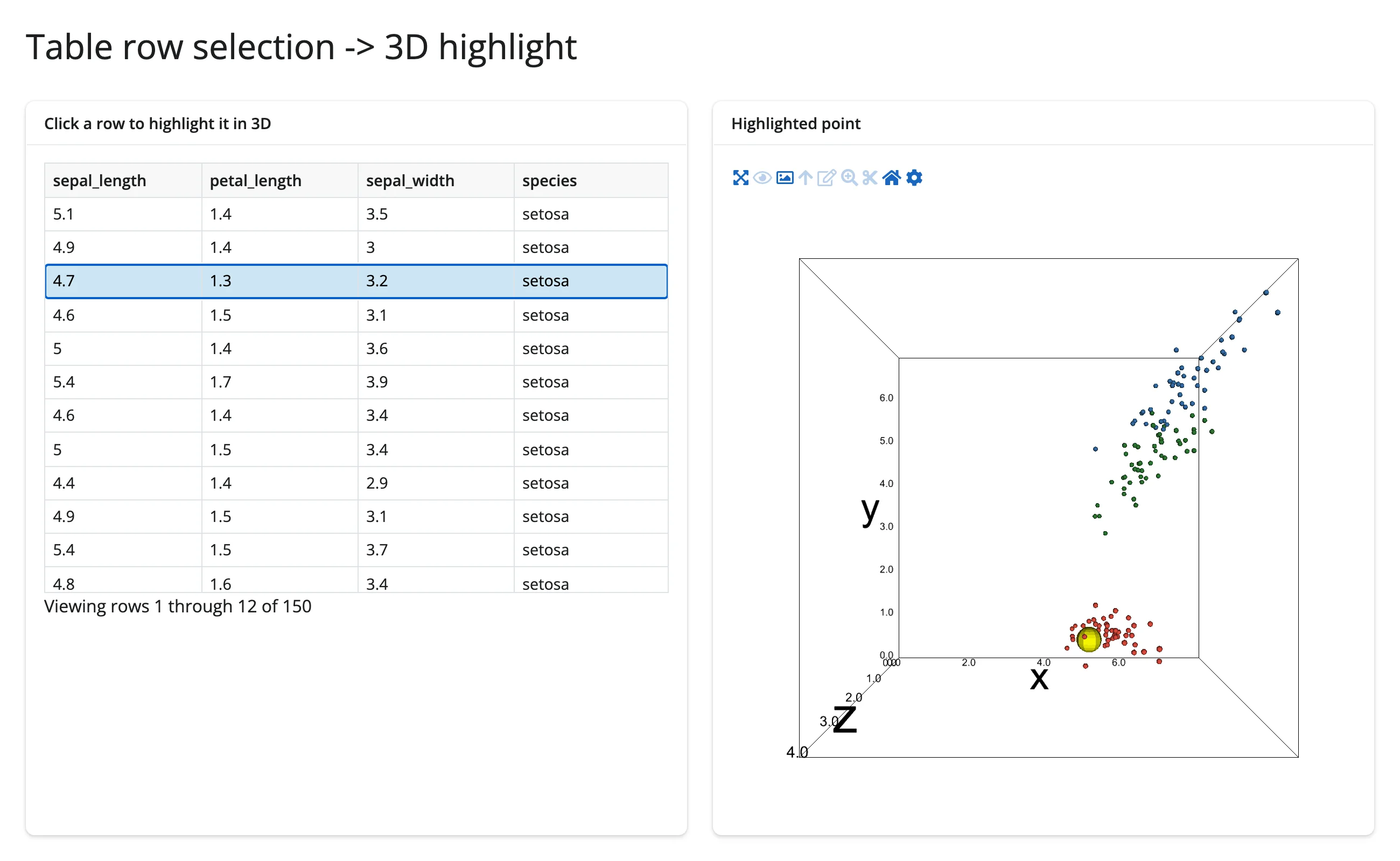
Clicking a second, different row relocates the highlight correctly – unlike ipyvolume’s native selected mechanism (see Gotchas), which gets stuck on the first point it ever highlights:

table moved

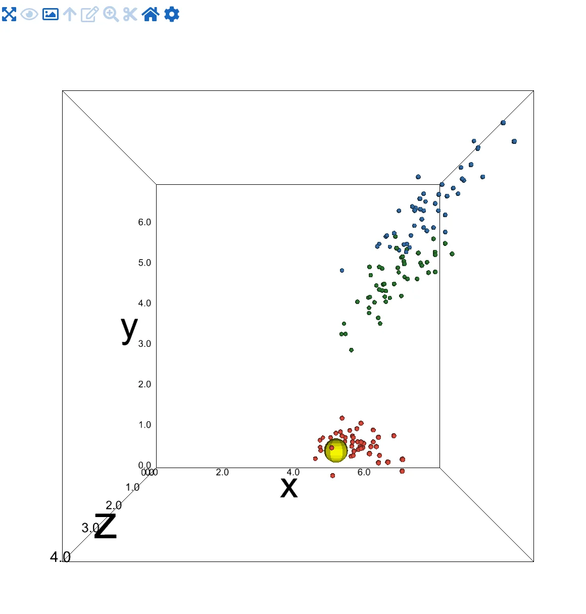
Because this recomputes the color/size arrays on every selection, the whole figure re-renders (the camera resets) – a reasonable trade for a table-driven highlight. Pairs with: itables, reactable, ipydatagrid (any table with row selection).

Animated sequence -> companion chart

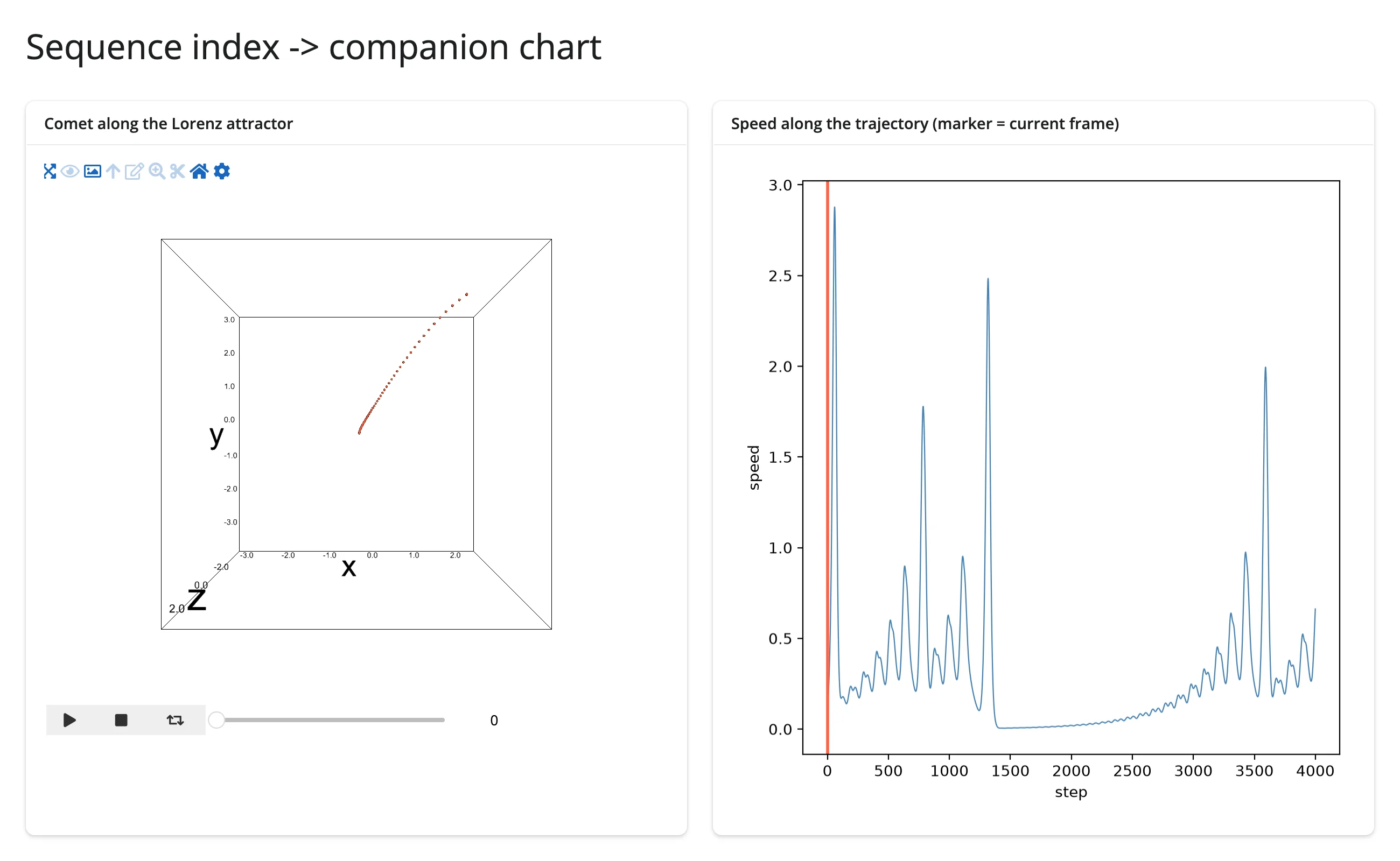
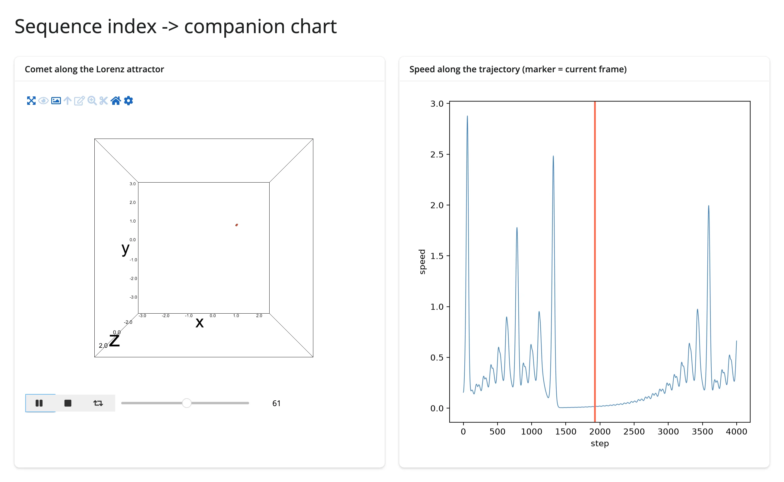
reactive_read(scatter, "sequence_index") turns the Play button’s current frame into a value a completely separate output can use – here, a vertical marker on a 2D speed chart that tracks a comet animating along a Lorenz attractor.

examples/12_sequence_linked_chart.py62 lines

import ipyvolume as ipv
import numpy as np
from shiny.express import render, ui

from shinywidgets import reactive_read, render_ipyvolume, render_widget

# Animated scatter driving a 2D companion chart: `sequence_index` isn't an
# accessor (ipyvolume has none for it), but it's an ordinary synced trait, so
# `reactive_read()` turns the Play button's current frame into a reactive
# value any other output can use -- here, a vertical marker on a speed chart.
ui.page_opts(title="Sequence index -> companion chart", fillable=True)


def lorenz(n=4000, dt=0.006, sigma=10.0, rho=28.0, beta=8 / 3):
    pts = np.empty((n, 3))
    p = np.array([1.0, 1.0, 1.0])
    for i in range(n):
        v = np.array([sigma * (p[1] - p[0]), p[0] * (rho - p[2]) - p[1], p[0] * p[1] - beta * p[2]])
        p += dt * v
        pts[i] = p
    speed = np.linalg.norm(np.gradient(pts, axis=0), axis=1)
    return pts, speed


pts, speed = lorenz()
xyz = (pts - pts.mean(axis=0)) / pts.std(axis=0)

S, TAIL = 120, 50
starts = np.linspace(0, len(xyz) - TAIL - 1, S).astype(int)
comet = np.stack([xyz[s : s + TAIL] for s in starts], axis=0).astype(np.float32)

with ui.layout_columns():
    with ui.card():
        ui.card_header("Comet along the Lorenz attractor")

        @render_ipyvolume
        def plot():
            fig = ipv.figure()
            ipv.scatter(comet[:, :, 0], comet[:, :, 1], comet[:, :, 2], size=1, marker="sphere", color="tomato")
            return fig

        @render_widget
        def controls():
            fig = plot.value
            if fig is None:
                return None
            return ipv.animation_control(fig.scatters[0], add=False, interval=50)

    with ui.card():
        ui.card_header("Speed along the trajectory (marker = current frame)")

        @render.plot
        def speed_chart():
            import matplotlib.pyplot as plt

            frame = reactive_read(plot.widget.scatters[0], "sequence_index")
            fig, ax = plt.subplots()
            ax.plot(speed, color="steelblue", linewidth=0.8)
            ax.axvline(starts[frame], color="tomato", linewidth=2)
            ax.set_xlabel("step")
            ax.set_ylabel("speed")
            return fig

Before pressing Play, the marker sits at step 0:

sequence before

A few seconds after pressing Play, the comet has moved and the marker has tracked it to the matching step:

sequence after

Large data

ipyvolume draws with the GPU (WebGL), so it’s the “draw it with the GPU in the browser” approach – see Large data & performance’s three approaches. Scatter/quiver markers are GPU-instanced and comfortable into the tens of thousands of points; volume rendering (ipyvolume.volshow) ray-marches a full 3D array in the browser, so its cost is dominated by texture upload size, not point count. For single-figure point clouds past 100k points, or voxel grids larger than a texture upload wants to carry, reach for k3d instead – it’s built for exactly that scale (see the guide’s intro for this comparison).

Layout and sizing

A figure’s WebGL canvas is resized to fill its container (and tracks later resizes) unless the figure has an explicit width/height – set via ipv.figure(width=..., height=...), Layout(height=...), or output_widget(height=...). An explicitly sized figure keeps its pixel size even inside a differently sized output (the output clips or pads it, rather than the output’s CSS stretching the canvas).

examples/13_layout_sizing.py32 lines

import ipyvolume as ipv
import numpy as np
from shiny.express import ui

from shinywidgets import render_ipyvolume

ui.page_opts(title="Layout and sizing", fillable=True)

rng = np.random.default_rng(0)
pts = rng.normal(size=(3, 500))


def make_fig(**kwargs):
    fig = ipv.figure(**kwargs)
    ipv.scatter(*pts, size=1, marker="sphere", color="tomato")
    return fig


with ui.layout_columns():
    with ui.card(full_screen=True):
        ui.card_header("Fills its card (try full_screen)")

        @render_ipyvolume
        def fill_plot():
            return make_fig()

    with ui.card():
        ui.card_header("Explicit figure size (400x300px): clipped, not stretched")

        @render_ipyvolume
        def fixed_plot():
            return make_fig(width=400, height=300)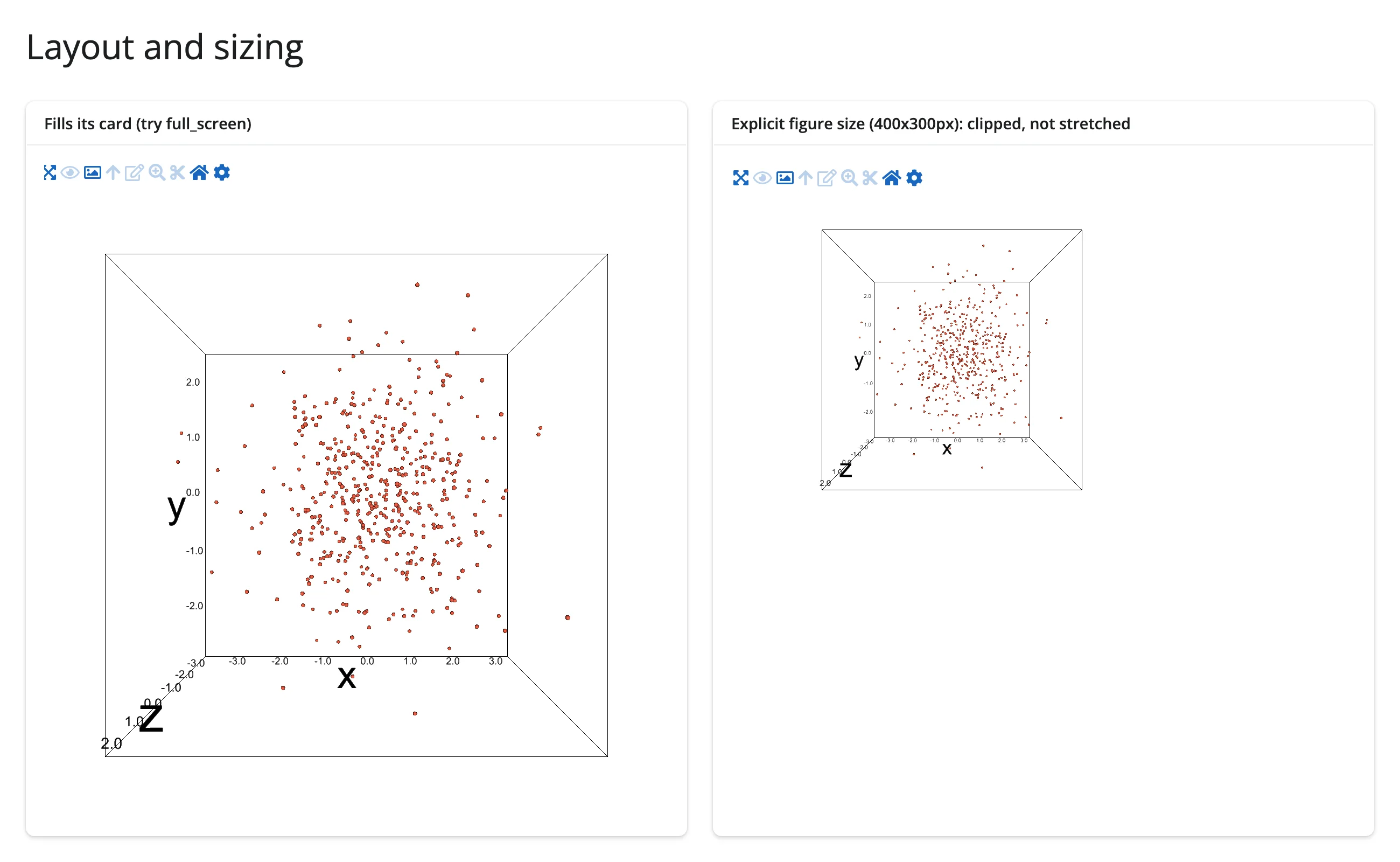

layout

full_screen=True on the card works as expected (the canvas grows to fill the expanded card and shrinks back on exit).

Gotchas and limitations

Verified against shinywidgets main @ 00f90249 (ipyvolume 0.6.3); all of the following are upstream ipyvolume bugs untouched by anything in the 00f90249..32ca7035 range (the accessor redesign, the comm-queue fix, and the pythreejs model-leak fix don’t reach this code), so they still apply on current main:

• A per-point array of color strings hangs the entire server process – not just that output. ipv.scatter(..., color=["tomato", "seagreen", ...]) (or any per-point array/list of multi-character strings) triggers an infinite loop in ipyvolume’s own color_to_binary_or_json() serializer the moment anything (a real Jupyter kernel too, not just shinywidgets) requests that scatter’s state. The whole server becomes unresponsive – a second, unrelated request to the same app also hangs. A solid color string (color="tomato") and a numeric (N, 3)/(N, 4) RGB(A) float array both work fine; only a per-point array of strings is broken. Always use a numeric RGB array for per-point coloring (every example above that colors by category does this).
• scatter.selected is broken for a repeatedly-updated highlight – two separate upstream bugs.
  1. Assigning selected to anything that serializes as an empty sequence (selected = [], the natural “nothing selected” state) crashes the view: ipyvolume’s frontend treats an empty array as truthy, then indexes it with i % 0 (NaN in JS), and a later .forEach() on the resulting undefined throws Cannot read properties of undefined (reading 'forEach'), blanking the figure. An out-of-range sentinel index (e.g. selected=[len(x)]) avoids this by never being empty. Filed upstream as ipyvolume#451. (2) Even with that sentinel, the highlight only ever reflects the first non-empty value selected is set to after a render: a second, different assignment changes the trait correctly (confirmed with reactive_read()) but the highlighted point never moves, with no error – not after a redraw-forcing orbit-drag or viewport resize. Both are upstream ipyvolume bugs in its own bundled frontend JS, not shinywidgets. Net effect: don’t use selected/size_selected/color_selected for a highlight that needs to change more than once. Bake it into plain color/size arrays instead (see Table row selection -> 3D highlight), which re-renders the figure but is verified correct across repeated, different selections.
• Lasso/rectangle selection is pixel-space only, not point indices. Set fig.selector = "rectangle" or "lasso" and register fig.on_selection(fn); the payload is {"type": ..., "pixel": [[x, y], ...]} – ipyvolume’s JS never computes which points fall inside the region. Mapping a browser selection back to data indices would mean reimplementing the camera frustum/polygon test yourself (the camera is available via camera(), so it’s possible, just not built in). scatter.selected is Python-to-browser only (and, per above, unreliable even for that): set it to highlight points you already know the indices of; it never reflects a user’s lasso back to you.
• Direct construction doesn’t auto-fit axes. ipv.Figure() defaults to a [0, 1]^3 box with nothing clipped or reframed; pylab drawing functions (ipv.scatter(), ipv.quiver(), ipv.plot_surface(), …) call _grow_limits() for you, but if you build Scatter/Mesh objects directly and assign them to fig.scatters, set fig.xlim/ylim/zlim explicitly (see the gallery showcase).
• Direct Scatter construction needs size_selected/color_selected set explicitly. Their trait defaults are 0-d numpy arrays, which don’t JSON-serialize; the pylab functions set sensible defaults for you, but a bare ipyvolume.widgets.Scatter(...) does not.
• size is a percentage of the viewport, not pixels. size=2 is roughly 20px on a 1000px-tall canvas; dense clouds usually want size in the 0.2-1 range. Points also balloon as the camera gets close (that’s the 3D perspective, not a bug).
• ipyvolume is unmaintained since 2023 (last release 0.6.3). It still renders correctly on current ipywidgets, but don’t expect upstream fixes for anything above, including the color-array hang.
• An upstream docs nit, not worth a workaround beyond awareness: the pylab scatter()/quiver()/etc. functions document a selection= keyword for setting initial indices; it’s a no-op on 0.6.3 (the real trait is selected, and the kwarg is silently dropped). Use selected= directly if you need to set it at construction time (but see the selected-after-render gotcha above before using it reactively).

What’s not a gotcha, despite an earlier internal report flagging it: pylab-style re-renders (rebuilding a figure with ipv.figure() + ipv.scatter() on every reactive invalidation) used to stall for ~29 seconds on alternating re-renders, caused by ipyvue/ipyvuetify template widgets shared across figures being closed by cleanup. That’s fixed on current main (process-global widgets now survive re-renders and sessions) – both pylab and direct construction re-render cleanly.

Gallery candidates

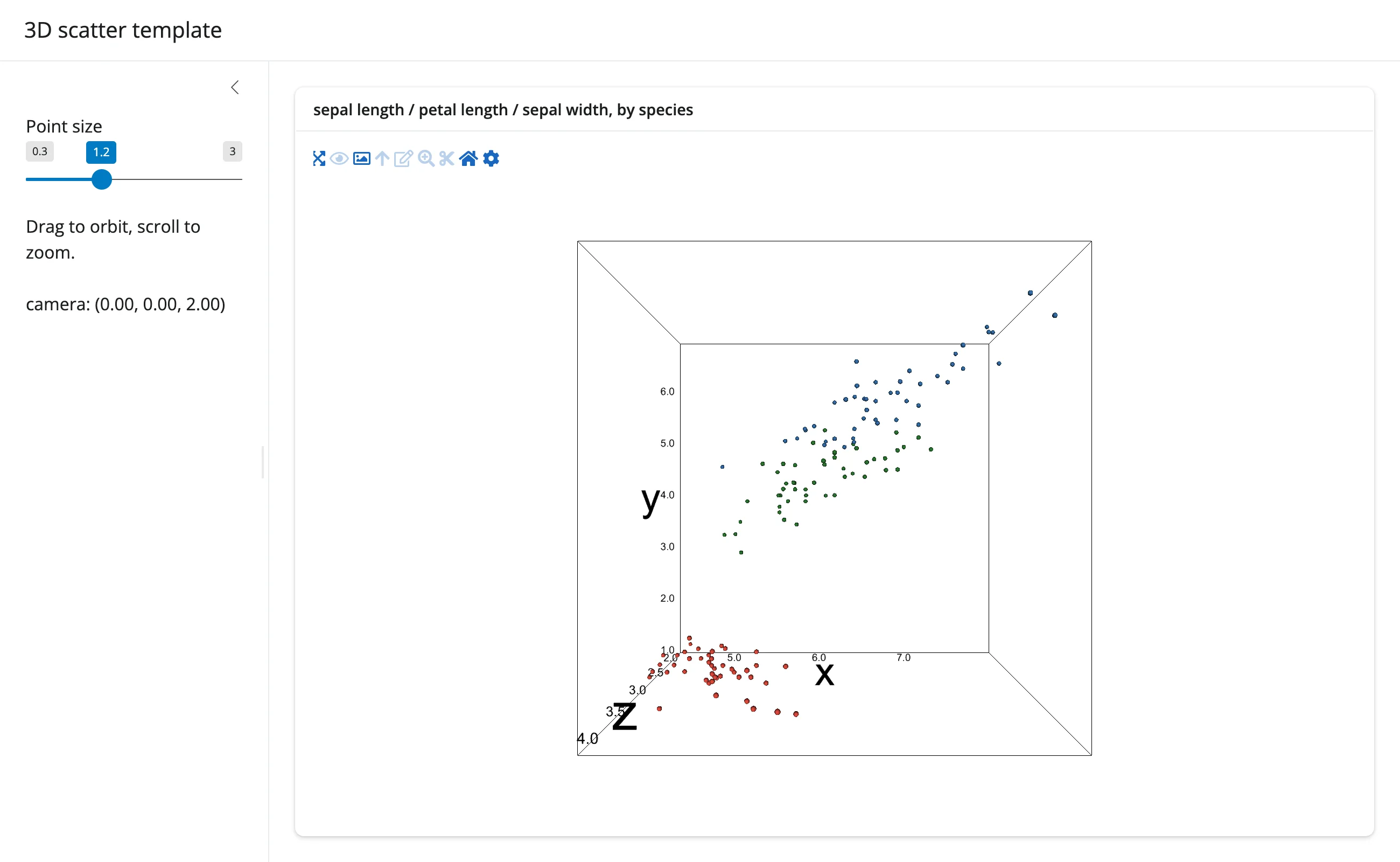
gallery/template_3d_scatter.py (template)

A clean starting point: direct construction with explicit axis limits, an in-place size slider, and a camera() readout in the sidebar – about 50 lines to adapt for your own 3D scatter.

template

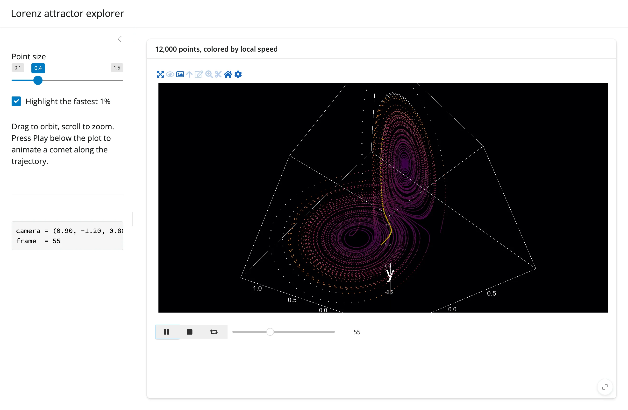
gallery/showcase_lorenz_explorer.py (showcase)

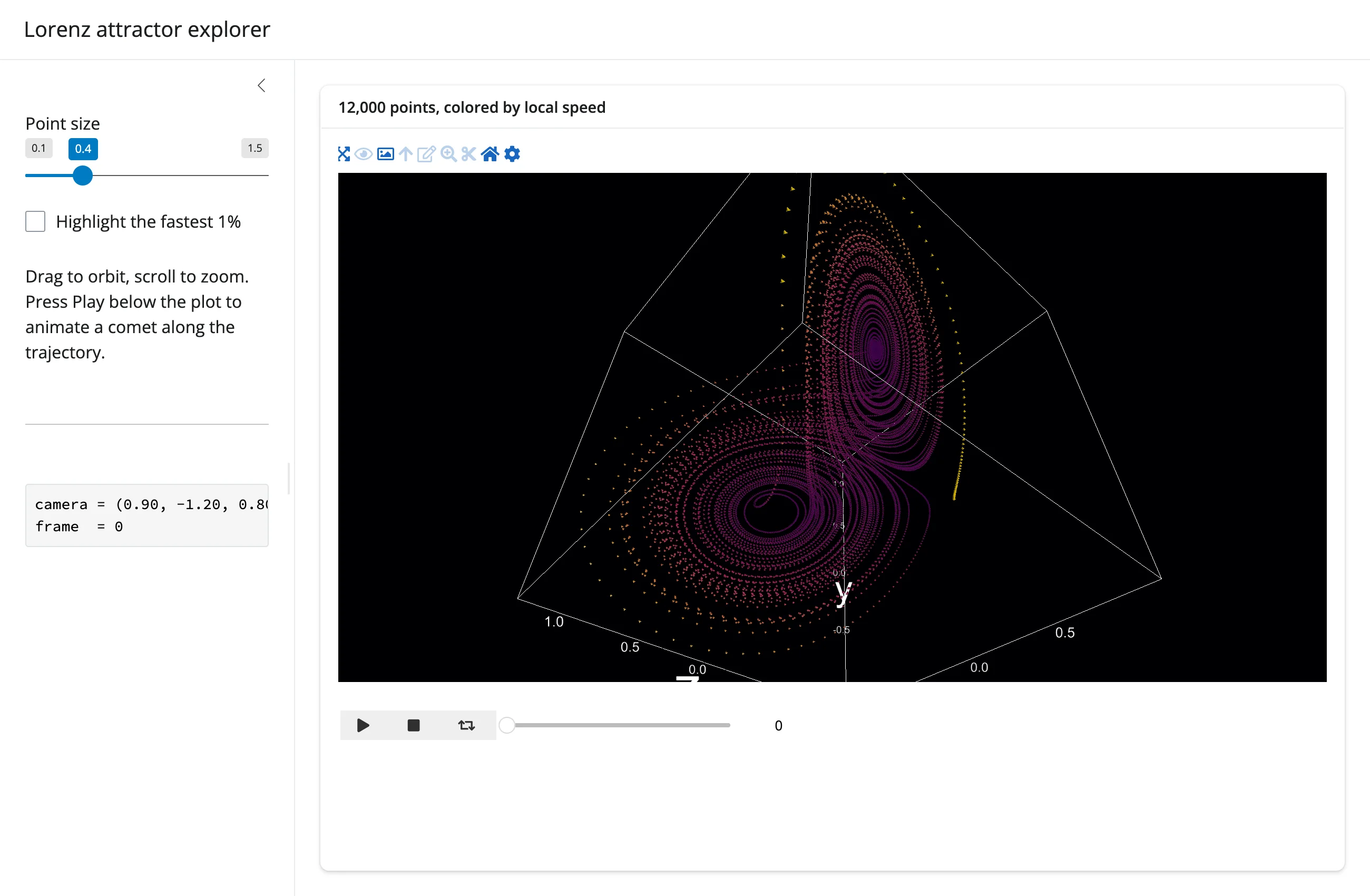
A numerically integrated Lorenz attractor (12,000 points, colored by local speed) with: direct construction and explicit limits, a dark theme, an in-place size slider, an in-place “highlight the fastest 1%” toggle (plain color-array swap, not selected), ipv.animation_control() as a second output animating a comet along the trajectory, and a camera() + sequence_index readout in the sidebar.

Learn more

• ipyvolume documentation
• ipyvolume GitHub (dormant since 2023)
• Related guides in this roster: pythreejs (shares the camera() accessor and Camera type; richer scene-graph control), k3d (alternative 3D point cloud/mesh/volume renderer, different performance/feature trade-offs), render-widget (the generic @render_widget/reactive_read() patterns this guide builds on)