ipyleaflet

A fully interactive Leaflet map in Shiny – draw shapes, click features, and drag markers, all wired back to Python.

ipyleaflet is the Jupyter Widgets binding for Leaflet, the small, mature JavaScript mapping library that powers a large share of the web’s interactive maps. ipyleaflet is maintained as part of the Jupyter widgets ecosystem and gives you Leaflet’s whole toolbox as Python objects: tile layers and basemaps, markers and marker clustering, GeoJSON and choropleths, drawing tools, split-screen comparison, legends, and more – each one a widget with synced traits.

@render_ipyleaflet renders a function that returns an ipyleaflet.Map (or a subclass, such as leafmap’s leafmap.leafmap.Map). It fills its container in a filling layout unless the map has an explicit height, and it types .widget as a real ipyleaflet.Map so .zoom, .add(), and friends autocomplete and type-check. Five accessors – bounds(), zoom(), center(), clicked(), and drawn_features() – turn the map into a genuine Shiny input: pans, zooms, clicks, and drawn shapes all come back to Python as reactive values, no reactive_read() boilerplate required.

Reach for ipyleaflet when you want the map itself to be an input (draw a region, click a feature, read the viewport) with fine control over individual layers. For a point cloud with tens of thousands of rows, prefer lonboard (WebGL, GPU-accelerated). For vector tiles, 3D terrain, or a globe, see maplibre. If you want one high-level API across several of these engines, plus a ready-made toolbar and 100+ basemaps, see leafmap, whose default backend is ipyleaflet and shares these same five accessors. For local raster files (GeoTIFF/COG), pair ipyleaflet with localtileserver.

Installation

pip install 'shinywidgets[ipyleaflet]'

Quick start

A map is just an ipyleaflet.Map with layers added to it. This one centers on Union Square in Manhattan and drops a marker with a popup:

examples/01_quickstart.py16 lines

import ipywidgets
import ipyleaflet as L
from shiny.express import ui
from shinywidgets import render_ipyleaflet

ui.page_opts(title="ipyleaflet quickstart", fillable=True)

with ui.card():

    @render_ipyleaflet
    def map():
        m = L.Map(center=(40.73, -73.99), zoom=15)
        marker = L.Marker(location=(40.735, -73.991))
        marker.popup = ipywidgets.HTML("<b>Union Square</b><br>14th St &amp; Broadway")
        m.add(marker)
        return m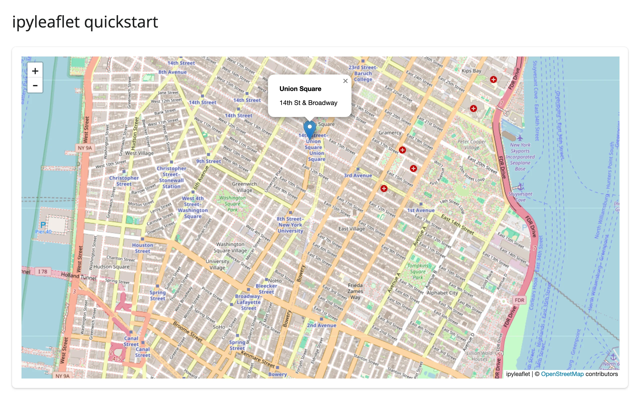

What you can build

Basemaps and layer switching

Any number of ipyleaflet.TileLayers can be marked base=True and listed in a LayersControl, which draws a radio-button picker. One quirk worth knowing up front: ipyleaflet doesn’t enforce exclusivity before the user interacts (see Gotchas), so add your intended default layer last.

examples/02_basemaps.py30 lines

import ipyleaflet as L
from shiny.express import ui
from shinywidgets import render_ipyleaflet

ui.page_opts(title="Basemaps", fillable=True)

with ui.card():

    @render_ipyleaflet
    def map():
        m = L.Map(center=(40.73, -73.99), zoom=12)  # default basemap: OSM Mapnik
        mapnik = m.layers[0]

        satellite = L.basemap_to_tiles(L.basemaps.Esri.WorldImagery)
        satellite.base, satellite.name = True, "Satellite"
        m.add(satellite)

        topo = L.basemap_to_tiles(L.basemaps.OpenTopoMap)
        topo.base, topo.name = True, "Topo"
        m.add(topo)

        m.add(L.LayersControl(position="topright"))

        # Every base=True layer stays visible until the user picks one in the
        # control (ipyleaflet doesn't enforce exclusivity up front), so
        # whichever was added last is what actually shows. Re-add the
        # intended default last so it's the one on top initially.
        m.remove(mapnik)
        m.add(mapnik)
        return m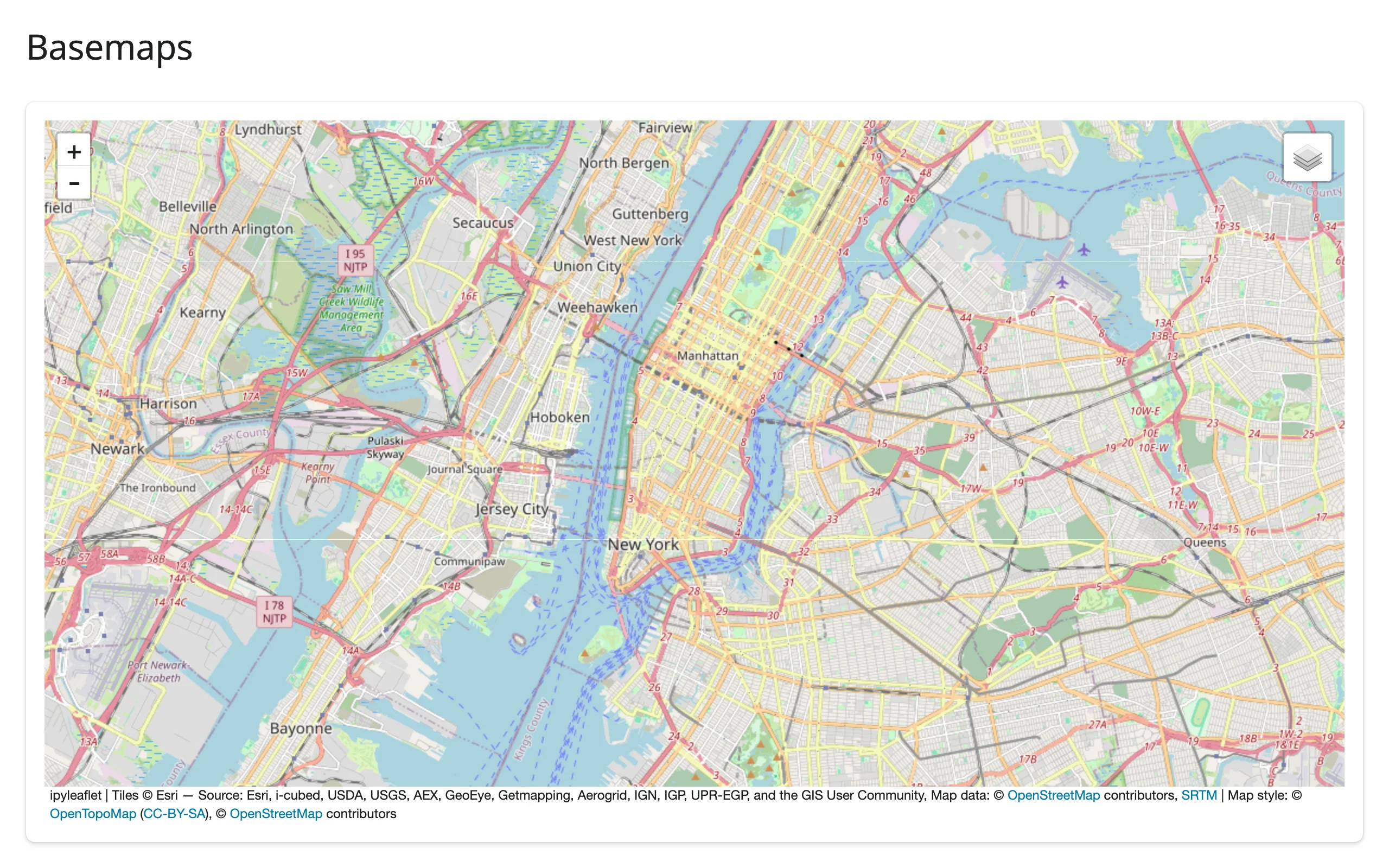

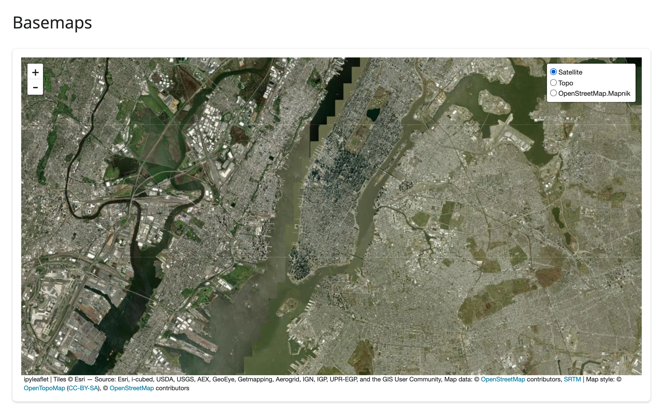
basemaps default basemaps satellite

Esri’s WorldImagery and OpenTopoMap are free; CARTO’s basemaps (CartoDB.Positron, etc.) now require an API key and render “API KEY REQUIRED” tiles without one.

Marker clustering

For more than a few hundred points, wrap Markers in a MarkerCluster so Leaflet groups nearby markers and only draws what’s visible. This map plots all 249 pods from plotly’s carshare sample dataset (real, anonymized car2go usage data for Montreal):

examples/03_markers_clusters.py18 lines

import ipyleaflet as L
import plotly.express as px
from shiny.express import ui
from shinywidgets import render_ipyleaflet

ui.page_opts(title="Marker clustering", fillable=True)

# plotly's carshare dataset: 249 real car2go pod locations around Montreal
pods = px.data.carshare()

with ui.card():

    @render_ipyleaflet
    def map():
        m = L.Map(center=(45.52, -73.59), zoom=11)
        markers = [L.Marker(location=(r.centroid_lat, r.centroid_lon)) for r in pods.itertuples()]
        m.add(L.MarkerCluster(markers=markers))
        return m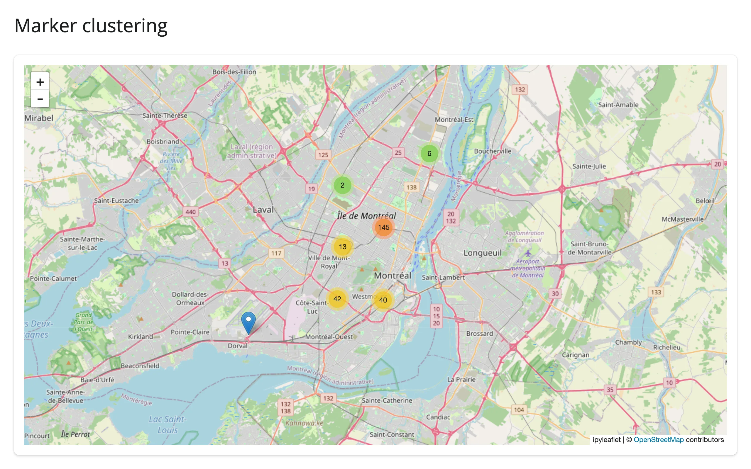

For thousands of points, a single GeoJSON layer (below) is dramatically cheaper to render and re-send than many Marker widgets – see Gotchas.

GeoJSON choropleth

ipyleaflet.Choropleth colors GeoJSON polygons by a value you supply, using a branca colormap. Here the same 249 pods are aggregated by total usage (car_hours) into a 5x5 grid:

examples/04_choropleth.py57 lines

import numpy as np
import ipyleaflet as L
import plotly.express as px
from branca.colormap import linear
from shiny.express import ui
from shinywidgets import render_ipyleaflet

ui.page_opts(title="GeoJSON choropleth", fillable=True)

# plotly's carshare dataset: 249 real car2go pod locations around Montreal,
# aggregated by total usage (car_hours) into a 5x5 grid of cells
pods = px.data.carshare()
lats, lons, hours = pods["centroid_lat"], pods["centroid_lon"], pods["car_hours"]

GRID = 5
lat_edges = np.linspace(lats.min(), lats.max(), GRID + 1)
lon_edges = np.linspace(lons.min(), lons.max(), GRID + 1)
i = np.clip(np.digitize(lats, lat_edges) - 1, 0, GRID - 1)
j = np.clip(np.digitize(lons, lon_edges) - 1, 0, GRID - 1)

features, choro_data = [], {}
for r in range(GRID):
    for c in range(GRID):
        cell_id = f"{r}-{c}"
        mask = (i == r) & (j == c)
        choro_data[cell_id] = float(hours[mask].sum())
        lon0, lon1 = lon_edges[c], lon_edges[c + 1]
        lat0, lat1 = lat_edges[r], lat_edges[r + 1]
        features.append(
            {
                "type": "Feature",
                "id": cell_id,
                "properties": {},
                "geometry": {
                    "type": "Polygon",
                    "coordinates": [
                        [[lon0, lat0], [lon1, lat0], [lon1, lat1], [lon0, lat1], [lon0, lat0]]
                    ],
                },
            }
        )

with ui.card():

    @render_ipyleaflet
    def map():
        m = L.Map(center=(45.52, -73.59), zoom=11)
        m.add(
            L.Choropleth(
                geo_data={"type": "FeatureCollection", "features": features},
                choro_data=choro_data,
                colormap=linear.YlOrRd_06,
                border_color="white",
                style={"fillOpacity": 0.75},
            )
        )
        return m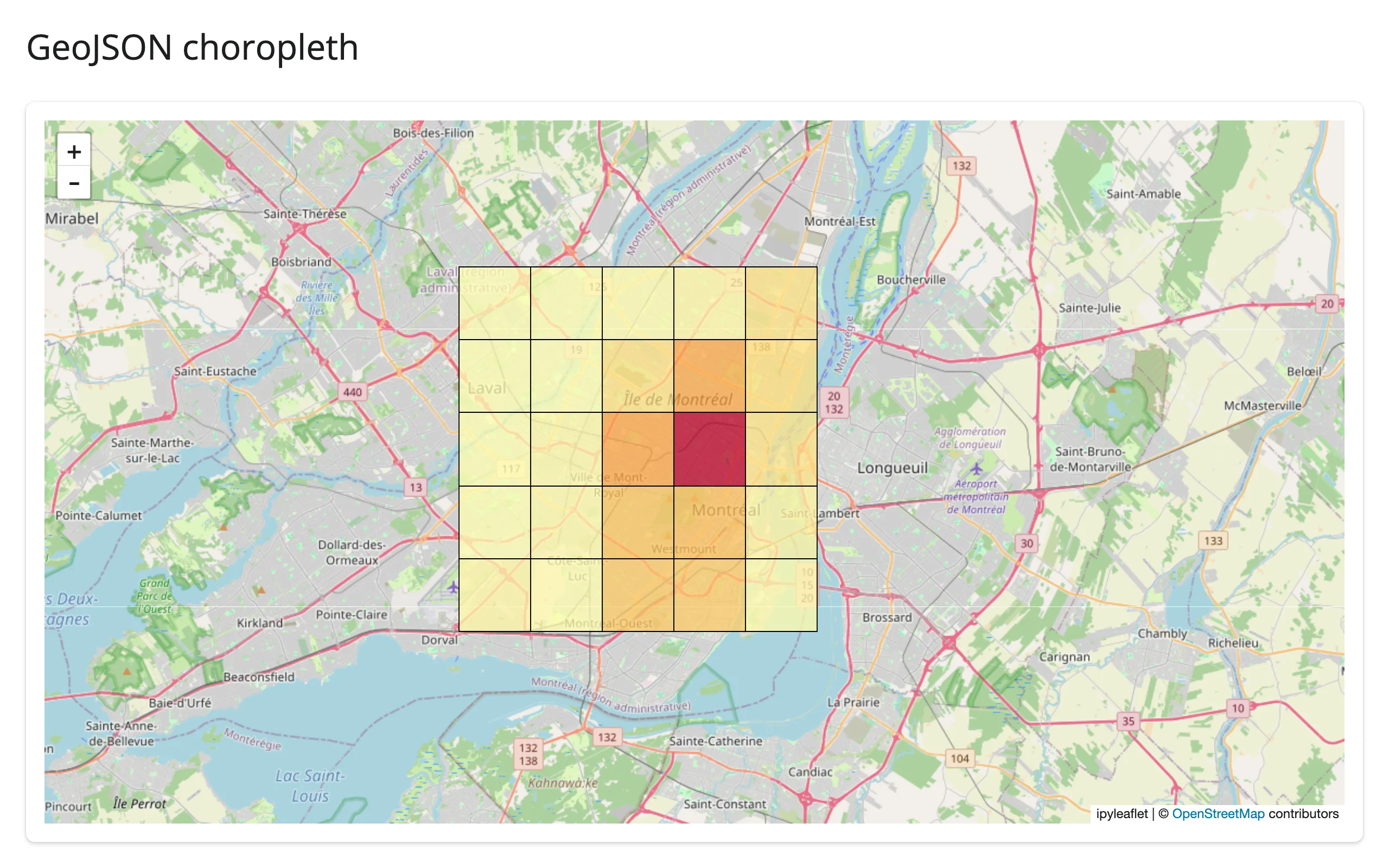

Drawing tools

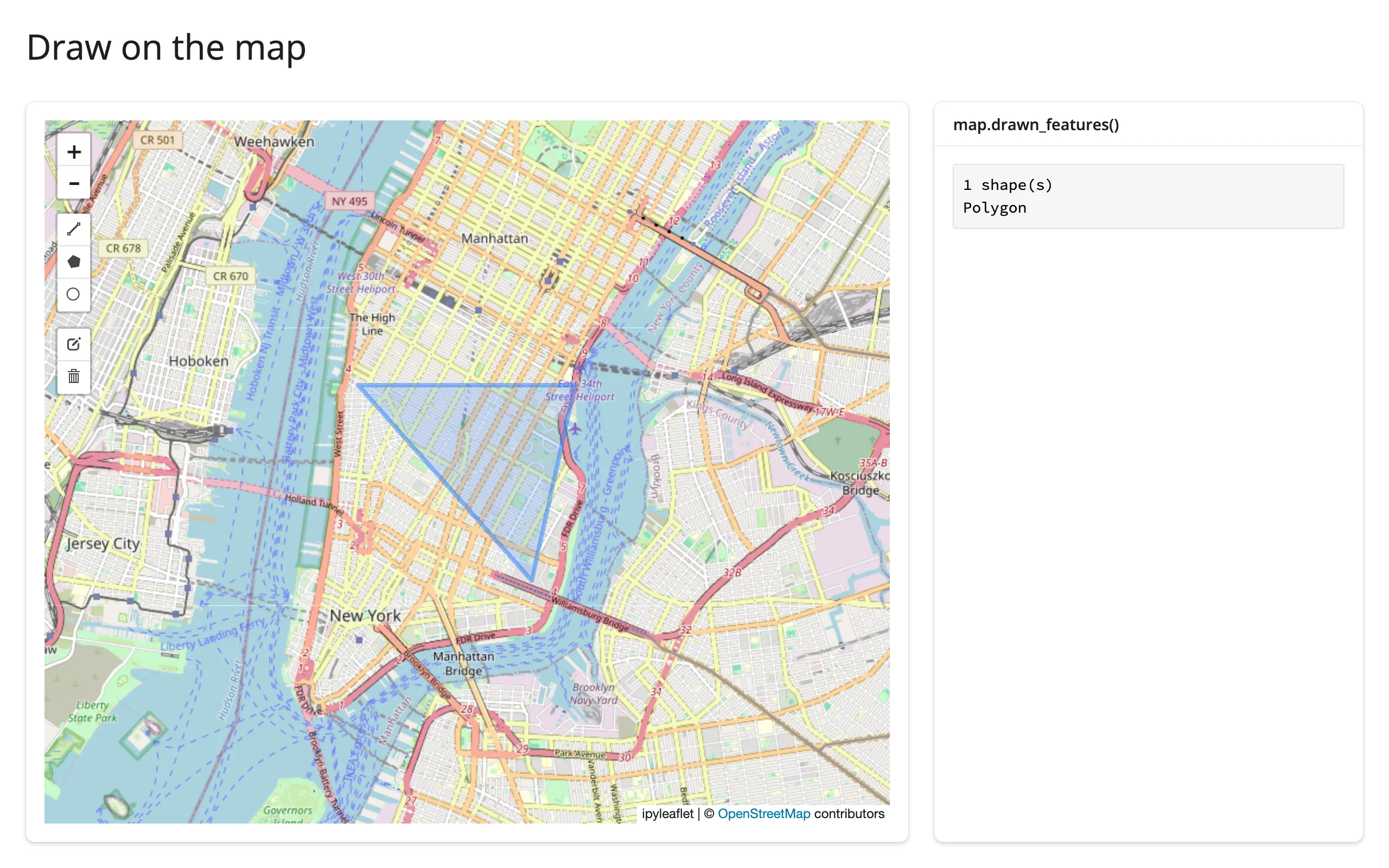
ipyleaflet.DrawControl adds a toolbar for drawing polygons, rectangles, circles, and markers directly on the map. Note the rectangle={"shapeOptions": {}} below – an empty dict ({}) disables a tool entirely, so to turn one on, give it a (possibly empty) shapeOptions, matching how polygon/polyline/circlemarker already default. This example also reads the shapes back with drawn_features(), covered in depth in the next section:

examples/05_draw_tool.py23 lines

import ipyleaflet as L
from shiny.express import render, ui
from shinywidgets import render_ipyleaflet

ui.page_opts(title="Draw on the map", fillable=True)

with ui.layout_columns(col_widths=[8, 4]):
    with ui.card():

        @render_ipyleaflet
        def map():
            m = L.Map(center=(40.73, -73.99), zoom=13)
            m.add(L.DrawControl(polygon={"shapeOptions": {"color": "#2a7fff"}}))
            return m

    with ui.card():
        ui.card_header("map.drawn_features()")

        @render.code
        def features():
            feats = map.drawn_features()
            kinds = [f["geometry"]["type"] for f in feats]
            return f"{len(feats)} shape(s)\n" + "\n".join(kinds)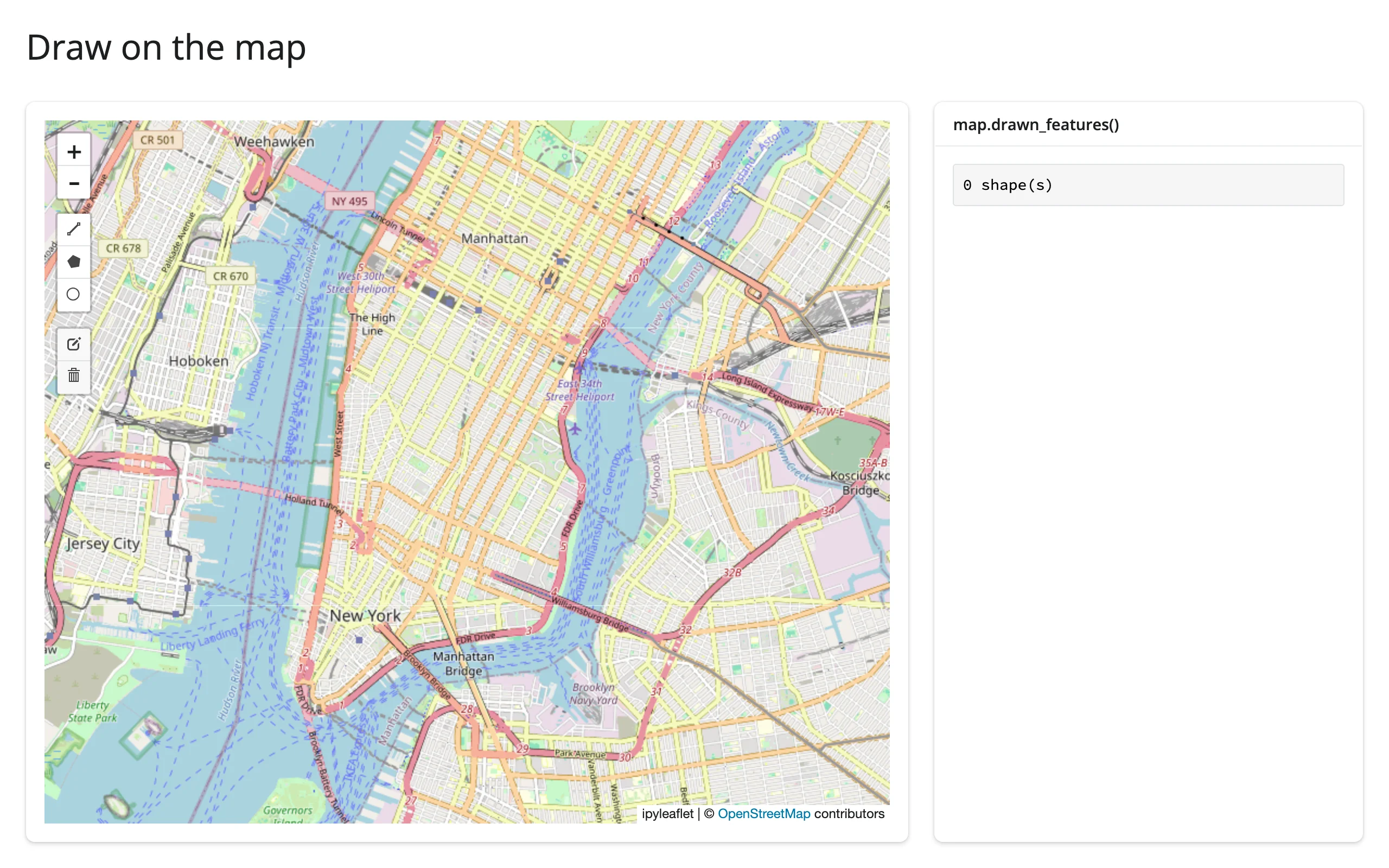

draw before draw after

Split-screen comparison

ipyleaflet.SplitMapControl puts two layers side by side with a draggable divider – useful for before/after imagery, two basemaps, or two time periods of the same data. Pass the two layers directly to the control; they aren’t also added to the map with m.add():

examples/15_split_map.py15 lines

import ipyleaflet as L
from shiny.express import ui
from shinywidgets import render_ipyleaflet

ui.page_opts(title="Split map comparison", fillable=True)

with ui.card():

    @render_ipyleaflet
    def map():
        m = L.Map(center=(40.73, -73.99), zoom=12)
        left = L.basemap_to_tiles(L.basemaps.OpenStreetMap.Mapnik)
        right = L.basemap_to_tiles(L.basemaps.Esri.WorldImagery)
        m.add(L.SplitMapControl(left_layer=left, right_layer=right))
        return m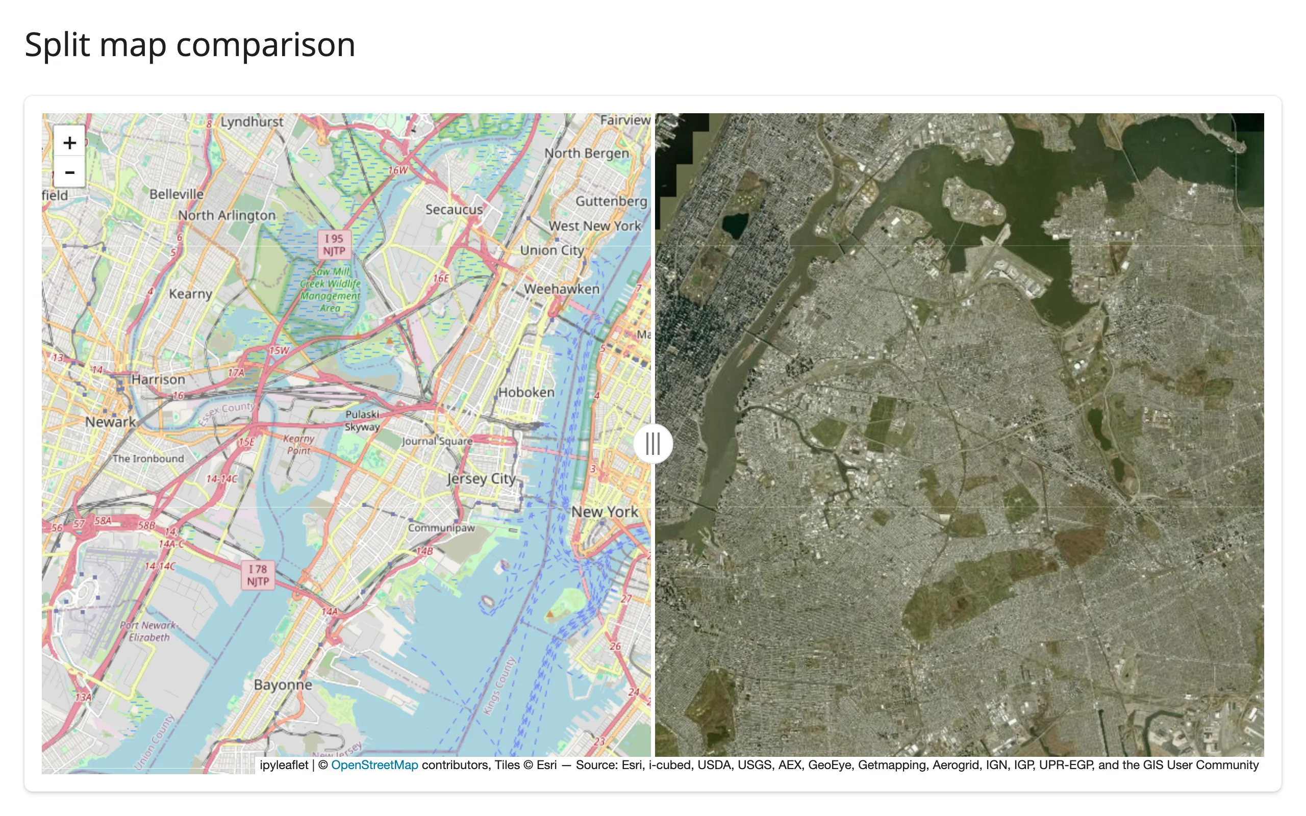

Reacting to user interaction

Accessor reference

Every accessor attaches the moment the map renders and records what the user does whether or not anything has read it yet – a click, pan, or drawn shape that happens before the first read still shows up in it.

accessor	returns	before any interaction	across re-render	default rate policy
`bounds()`	`((south, west), (north, east))`, `[lat, lng]` order	Cancels (like an unrendered output) until the browser’s first report	Re-seeded; cancels again until the new map reports	none
`zoom()`	`float`	Seeded (the map’s own `.zoom`)	Re-seeded from the new map	none
`center()`	`[lat, lng]`	Seeded (the map’s own `.center`)	Re-seeded from the new map	none
`clicked()`	`dict` with `coordinates: [lat, lng]` (and other native `on_interaction` kwargs)	`None` until the first click	Kept until the user clicks the new map	none
`drawn_features()`	`List[dict]` of GeoJSON Features	`[]` until something is drawn	Re-seeded (`[]` for a fresh `DrawControl`)	none

None of the five declares a default rate limit – see Rate limiting for why, and for when you’d add one yourself. Coordinates throughout are [lat, lng], as ipyleaflet reports them; lonboard and maplibre are (lng, lat).

bounds(), zoom(), center(), and drawn_features() describe the map’s own state, so a re-render – which builds a fresh Map – re-seeds them from the new map: zoom()/center() immediately reflect the new map’s constructor arguments, bounds() goes back to cancelling until the browser reports the new map’s viewport, and drawn_features() goes back to [] for the new map’s own (empty) DrawControl. clicked() is different: a click is something the user did, not something the map owns, so it survives a re-render and keeps reporting the previous click until the user clicks the new map.

Camera state: `bounds()`, `zoom()`, `center()`

These three track the map’s viewport. bounds() is the one with a catch: it’s () in the browser until the very first render completes, so reading it cancels (silently, like an output that hasn’t rendered yet) rather than returning an empty tuple – no req() guard needed. This example also shows the two-way sync pattern: a slider sets .zoom on the widget, and zoom() (which also fires on that Python-side set) mirrors it back, without a feedback loop – update_slider() to a value the slider already holds doesn’t re-fire the input:

examples/06_camera_state.py41 lines

import ipyleaflet as L
from shiny import reactive
from shiny.express import input, render, ui
from shinywidgets import render_ipyleaflet

ui.page_opts(title="Camera accessors", fillable=True)

with ui.sidebar():
    ui.input_slider("zoom", "Zoom", value=12, min=4, max=18)

with ui.card():

    @render_ipyleaflet
    def map():
        return L.Map(center=(40.73, -73.99), zoom=12)


@reactive.effect
def _slider_to_map():
    map.widget.zoom = input.zoom()


@reactive.effect
def _map_to_slider():
    # zoom() also fires when Python sets .zoom (the line above), but the
    # slider ignores an update to the value it already holds, so this
    # doesn't loop
    ui.update_slider("zoom", value=map.zoom())


with ui.card(fill=False):

    @render.code
    def status():
        b = map.bounds()  # cancels (no output) until the browser first reports it
        return (
            f"zoom:   {map.zoom()}\n"
            f"center: {[round(c, 3) for c in map.center()]}\n"
            f"bounds: south={b[0][0]:.3f} west={b[0][1]:.3f} "
            f"north={b[1][0]:.3f} east={b[1][1]:.3f}"
        )

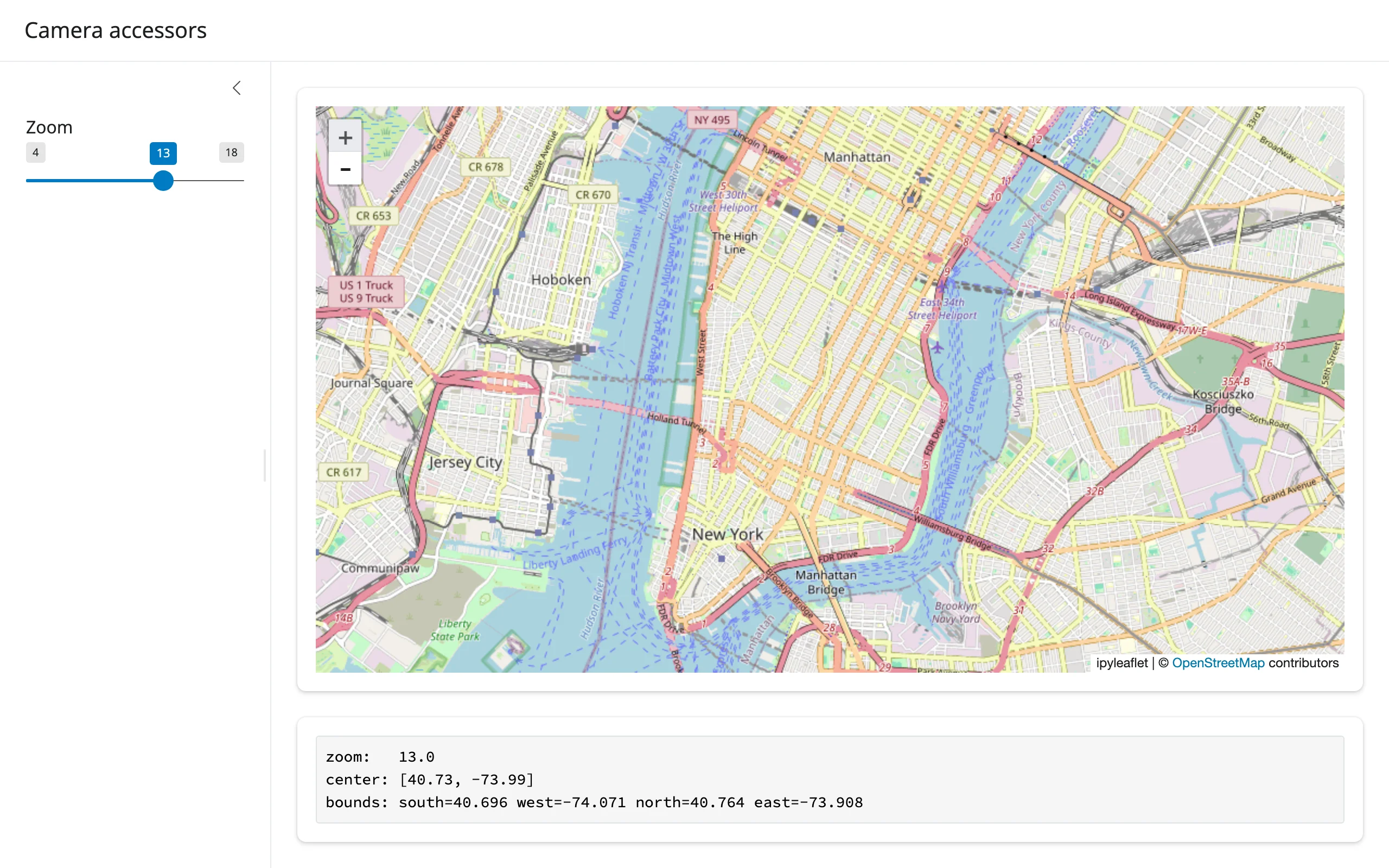
Verified: clicking the zoom-in control moved the slider from 12 to 13 and updated bounds/center in the status box, in one Playwright pass.

Clicks: `clicked()`

examples/07_clicked.py23 lines

import ipyleaflet as L
from shiny.express import render, ui
from shinywidgets import render_ipyleaflet

ui.page_opts(title="Map clicks", fillable=True)

with ui.layout_columns(col_widths=[8, 4]):
    with ui.card():

        @render_ipyleaflet
        def map():
            return L.Map(center=(40.73, -73.99), zoom=13)

    with ui.card():
        ui.card_header("map.clicked()")

        @render.code
        def click():
            c = map.clicked()
            if c is None:
                return "Click the map to see its coordinates."
            lat, lng = c["coordinates"]
            return f"lat={lat:.4f}\nlng={lng:.4f}"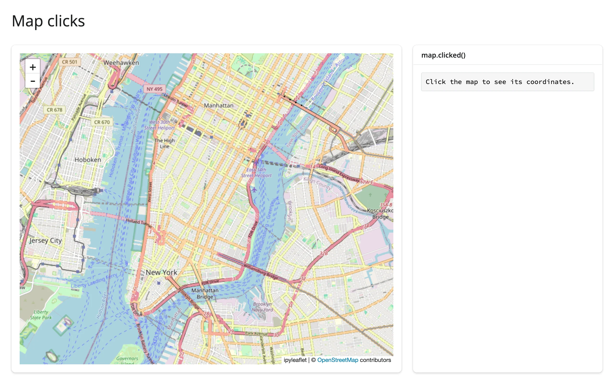

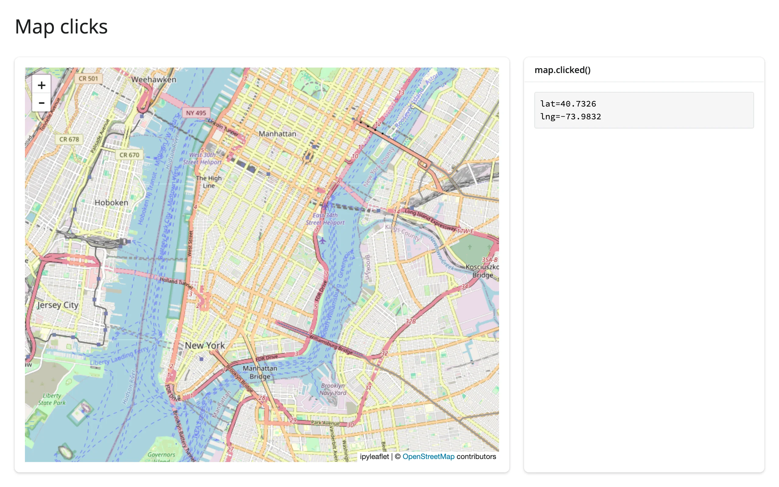
clicked before clicked after

Verified with a real click in Chromium. clicked() is kept across a re-render: click the map, trigger a re-render some other way (e.g. a sidebar input the map doesn’t depend on), and the previous click’s coordinates are still there until the user clicks the new map – verified by forcing a re-render after a click and confirming the value survives. Two more things worth knowing: a double-click sends two native click events plus a dblclick (which is ignored), but because both clicks of a double-click land on the same coordinate and clicked() is deduplicated like any other input (identical consecutive values don’t re-publish), a reader only sees one update per double-click in practice, not two. Second: marker clicks don’t bubble up to clicked() – use a layer’s own on_click (e.g. GeoJSON.on_click) for those.

Drawn shapes: `drawn_features()`

The same app as the drawing-tools example above demonstrates the accessor directly: map.drawn_features() returns [] until something is drawn, then a list of GeoJSON Feature dicts that updates as shapes are added, edited, or deleted. If the map has no ipyleaflet.DrawControl, reading it raises TypeError (add one with m.add(DrawControl())). See examples/05_draw_tool.py and its screenshots above – verified by actually drawing a triangle with Playwright mouse events (click each vertex, double-click to finish) and confirming the count and geometry type.

Reading on demand

Because every accessor attaches at render, a button, download handler, or chat/LLM tool callback can read one with no warm-up: nothing else needs to have read bounds() or drawn_features() first to keep them live. A “Save view” button is the simplest version of this pattern – capture the camera and any drawn shapes the instant the user asks, not continuously:

examples/16_read_on_demand.py40 lines

import ipyleaflet as L
from shiny import reactive
from shiny.express import input, render, ui
from shinywidgets import render_ipyleaflet

ui.page_opts(title="Save the current view on demand", fillable=True)

# Every accessor attaches when the map renders, so nothing needs to keep
# reading bounds()/drawn_features() for this button's reads to see the
# user's latest pan or shape -- they're there the moment the button is
# clicked, with no warm-up read required first.
saved = reactive.value([])

with ui.layout_columns(col_widths=[8, 4]):
    with ui.card():
        ui.input_action_button("save", "Save current view", class_="mb-2")

        @render_ipyleaflet
        def map():
            m = L.Map(center=(40.73, -73.99), zoom=13)
            m.add(L.DrawControl(polygon={"shapeOptions": {"color": "#2a7fff"}}))
            return m

    with ui.card():
        ui.card_header("Saved views")

        @render.ui
        def views():
            if not saved():
                return "Pan the map, maybe draw a shape, then click Save."
            items = [
                ui.tags.li(f"center={c} zoom={z:.0f} shapes={n}") for c, z, n in saved()
            ]
            return ui.tags.ol(*items)


@reactive.effect
@reactive.event(input.save)
def _save_view():
    saved.set([*saved(), (map.center(), map.zoom(), len(map.drawn_features()))])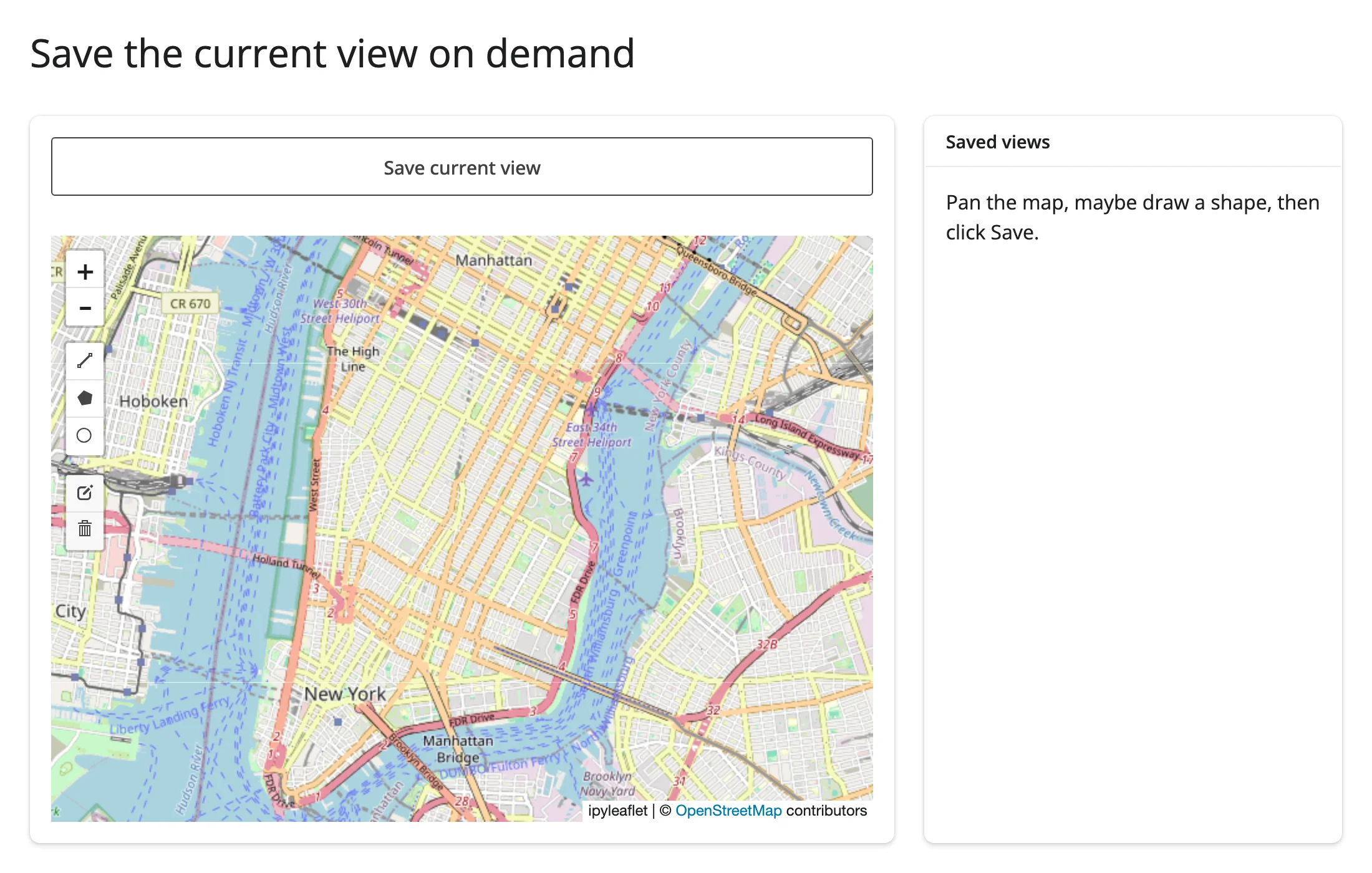

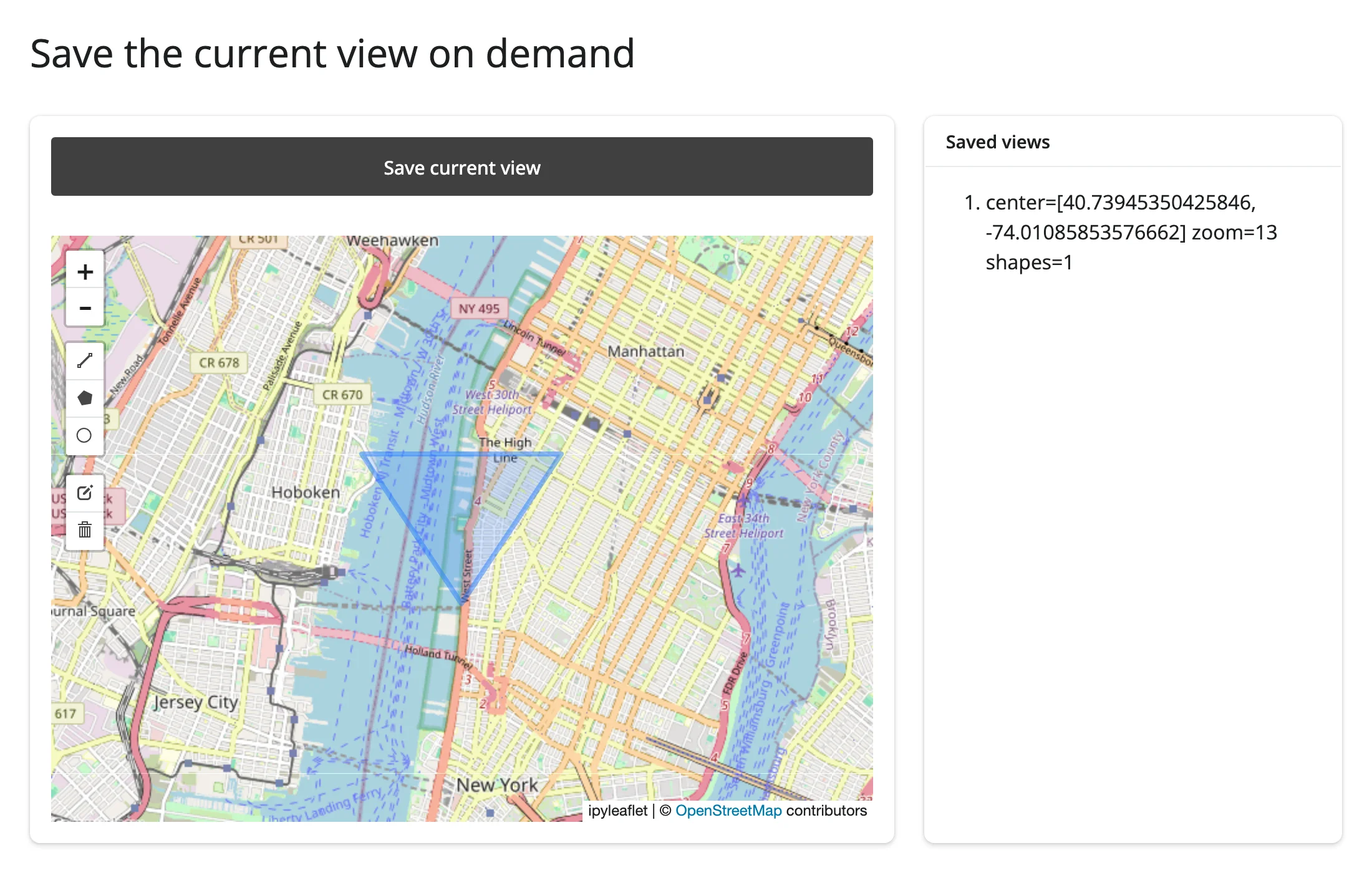
read on demand before read on demand after

Verified: pan the map, draw a triangle, click Save once – the saved entry has the panned-to center, the zoom level, and shapes=1, all read inside the button’s own @reactive.event handler with nothing else subscribed to center()/zoom()/drawn_features() elsewhere in the app.

Beyond the accessors: `reactive_read`

The accessors cover the map itself. For state on individual layers and controls – a draggable marker’s position, a GeoJSON layer’s hover state, anything not in the accessor table – use reactive_read() directly on the layer object. A layer or control isn’t the output’s own .widget, so there’s no .read() for it; reactive_read() is the tool for any child widget:

examples/08_reactive_read_marker_drag.py25 lines

import ipyleaflet as L
from shiny import req
from shiny.express import render, ui
from shinywidgets import reactive_read, render_ipyleaflet

ui.page_opts(title="Draggable marker (reactive_read)", fillable=True)

with ui.layout_columns(col_widths=[8, 4]):
    with ui.card():

        @render_ipyleaflet
        def map():
            m = L.Map(center=(40.73, -73.99), zoom=14)
            m.add(L.Marker(location=(40.73, -73.99), draggable=True, name="me"))
            return m

    with ui.card():
        ui.card_header("Drag the marker")

        @render.code
        def location():
            req(map.widget)
            marker = next(lyr for lyr in map.widget.layers if lyr.name == "me")
            lat, lng = reactive_read(marker, "location")
            return f"lat={lat:.4f}\nlng={lng:.4f}"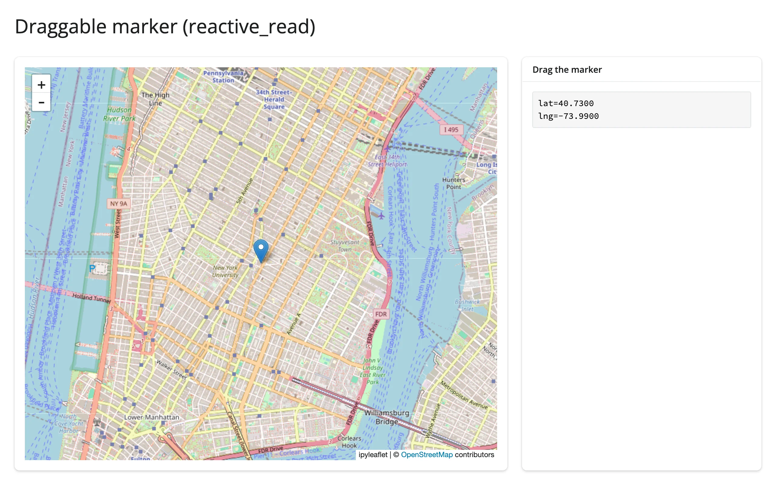

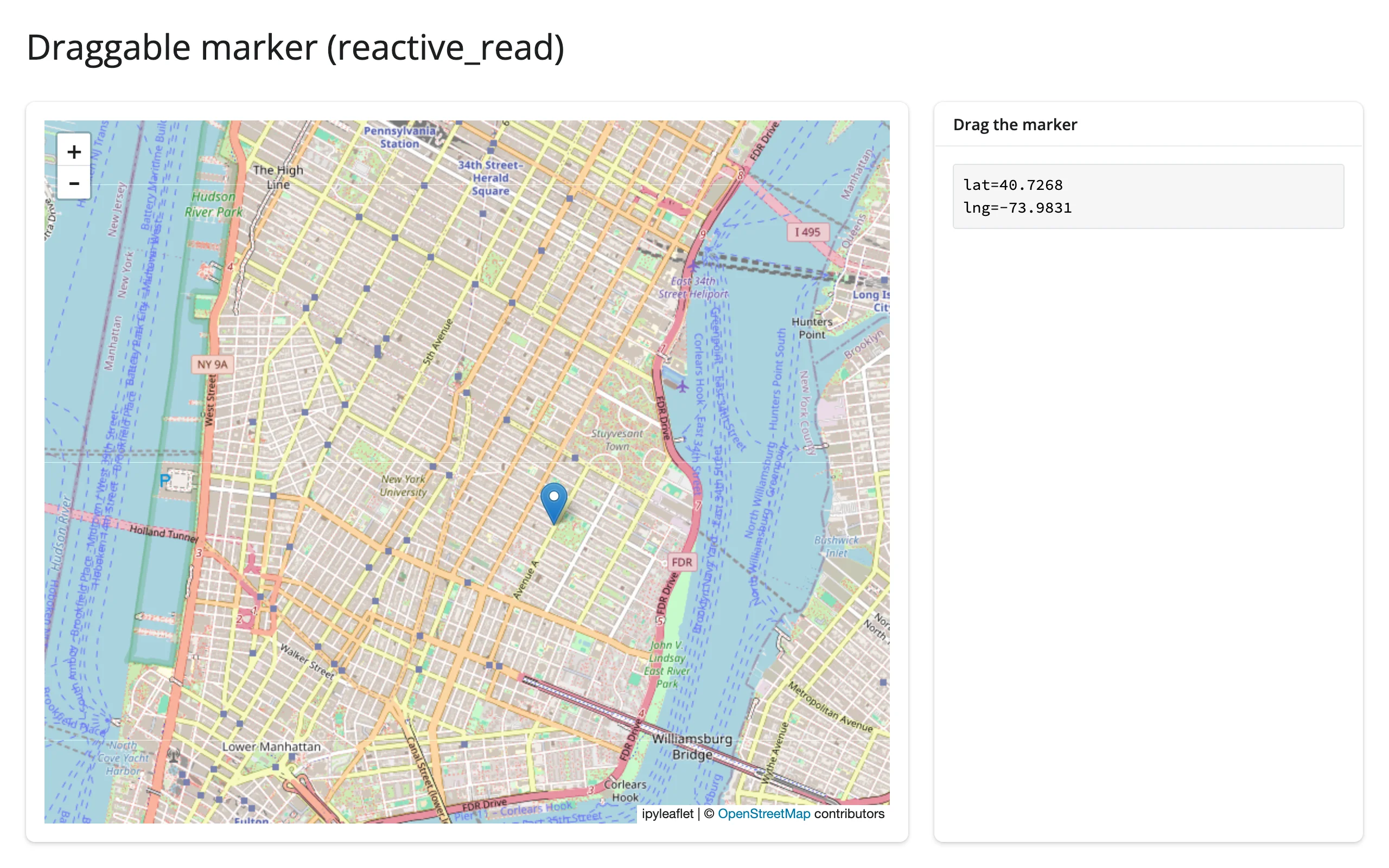
marker drag before marker drag after

Verified by dragging the marker with Playwright mouse events; the reported coordinates moved from the marker’s starting location to the drop point. Other useful traits to reactive_read(): a GeoJSON layer’s hover_style interactions via on_hover, and any DrawControl’s last_action/last_draw for more detail than drawn_features() exposes.

Rate limiting

None of ipyleaflet’s five accessors declare a default rate_policy – each only fires once per user gesture (one bounds()/zoom()/center() update per pan or zoom, one clicked() per click, one drawn_features() update per edit), so there’s nothing to smooth. The rate_policy/rate_delay parameters on @render_ipyleaflet instead govern reactive_read() on the widget, which matters for traits that do stream many updates per gesture – a dragged marker’s location fires continuously, not once at drop:

examples/09_rate_limiting.py38 lines

import ipyleaflet as L
from shiny import reactive, req
from shiny.express import render, ui
from shinywidgets import reactive_read, render_ipyleaflet

ui.page_opts(title="Rate-limited reactive_read", fillable=True)

# ipyleaflet's own accessors (bounds/zoom/center/clicked/drawn_features) only
# ever fire once per gesture, so rate_policy/rate_delay has nothing to smooth
# there. It matters for reactive_read() on a trait that streams many updates
# per gesture, like a dragged marker's "location".
with ui.layout_columns(col_widths=[8, 4]):
    with ui.card():

        @render_ipyleaflet(rate_policy="throttle", rate_delay=0.5)
        def map():
            m = L.Map(center=(40.73, -73.99), zoom=14)
            m.add(L.Marker(location=(40.73, -73.99), draggable=True, name="me"))
            return m

    with ui.card():
        ui.card_header("Drag updates seen by Python (throttled to 2/s)")
        count = reactive.value(0)

        @reactive.effect
        def _count():
            req(map.widget)
            marker = next(lyr for lyr in map.widget.layers if lyr.name == "me")
            reactive_read(marker, "location")
            # isolate(): count() is both read and set here, so without
            # isolating the read this effect would depend on its own output
            # and loop forever instead of running once per throttled update
            with reactive.isolate():
                count.set(count() + 1)

        @render.code
        def n():
            return str(count())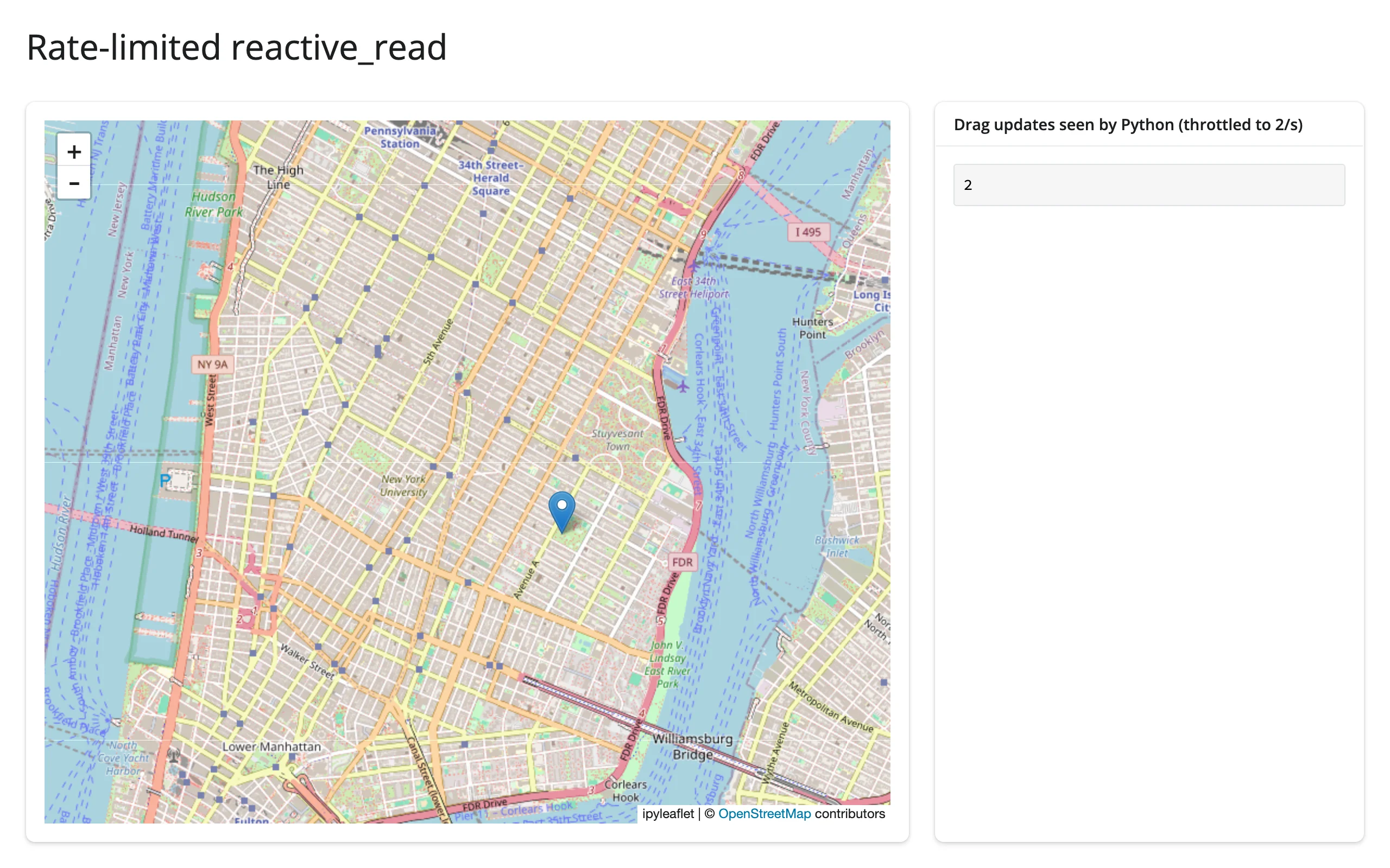

Verified with a 30-step Playwright drag: the throttle (0.5 s window) brought it down to 2 effect runs. Note the reactive.isolate() around count.set(count() + 1) – without it, this effect reads and writes the same reactive.Value in one body, which makes it depend on its own output and re-run forever, freezing the whole session (the map and every other output stop updating, with no error printed). This is a generic Shiny footgun, not specific to ipyleaflet, but it’s easy to hit the first time you wire up a counter like this.

Updating the widget from Python

Mutate map.widget’s layers and traits from a @reactive.effect instead of re-rendering: the browser patches just the layer that changed, the map keeps its current pan and zoom (and any shapes the user has drawn), and nothing re-sends the base widget bundle. This example toggles a layer’s visibility, restyles it, and swaps the basemap, all in place:

examples/10_inplace_updates.py57 lines

import ipyleaflet as L
from shiny import reactive
from shiny.express import input, ui
from shinywidgets import render_ipyleaflet

ui.page_opts(title="In-place layer updates", fillable=True)

OUTLINE = {
    "type": "Feature",
    "properties": {},
    "geometry": {
        "type": "Polygon",
        "coordinates": [
            [[-74.00, 40.72], [-73.98, 40.72], [-73.98, 40.74], [-74.00, 40.74], [-74.00, 40.72]]
        ],
    },
}

with ui.sidebar():
    ui.input_checkbox("show_outline", "Show outline", True)
    ui.input_radio_buttons("color", "Outline color", ["blue", "red", "green"])
    ui.input_checkbox("satellite", "Satellite basemap", False)

with ui.card():

    @render_ipyleaflet
    def map():
        m = L.Map(center=(40.73, -73.99), zoom=13)
        m.add(L.GeoJSON(data=OUTLINE, style={"color": "blue", "fillOpacity": 0.1}, name="outline"))
        return m


def outline():
    return next(lyr for lyr in map.widget.layers if lyr.name == "outline")


# Each effect mutates a trait on the already-rendered map, so the browser
# patches the one layer that changed instead of rebuilding the whole map --
# the pan/zoom the user has done is never disturbed.
@reactive.effect
def _toggle_outline():
    outline().visible = input.show_outline()


@reactive.effect
def _restyle_outline():
    outline().style = {**outline().style, "color": input.color()}


@reactive.effect
def _swap_basemap():
    m = map.widget
    old = next(lyr for lyr in m.layers if lyr.base)
    basemap = L.basemaps.Esri.WorldImagery if input.satellite() else L.basemaps.OpenStreetMap.Mapnik
    new = L.basemap_to_tiles(basemap)
    new.base = True
    m.substitute(old, new)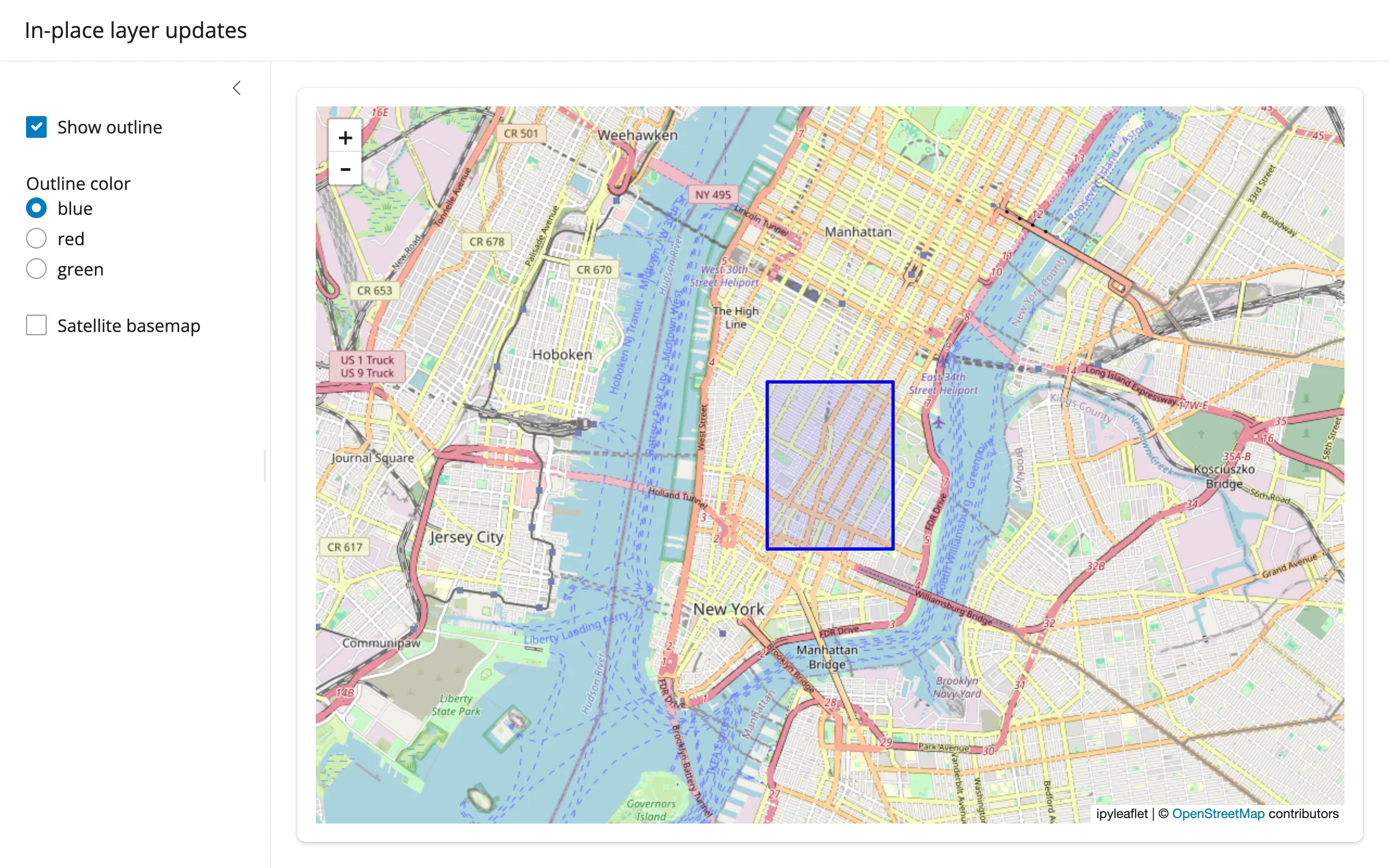

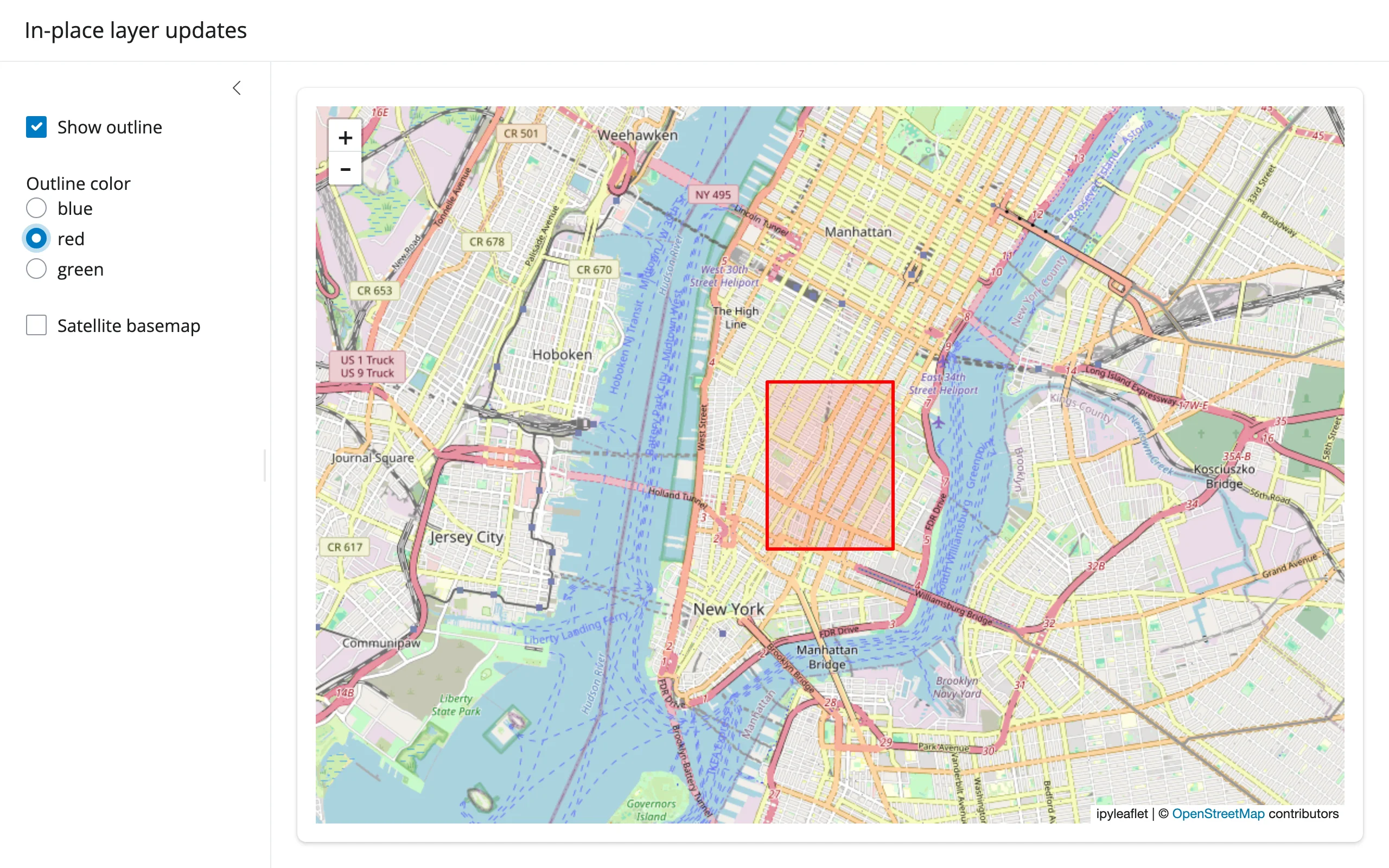
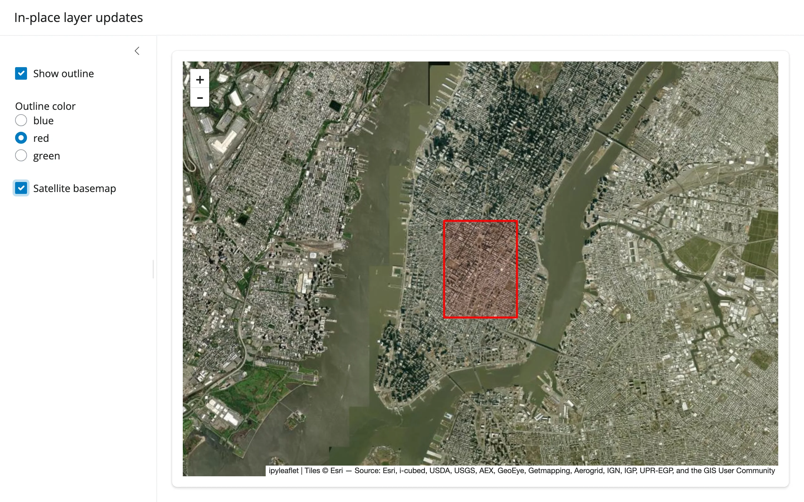
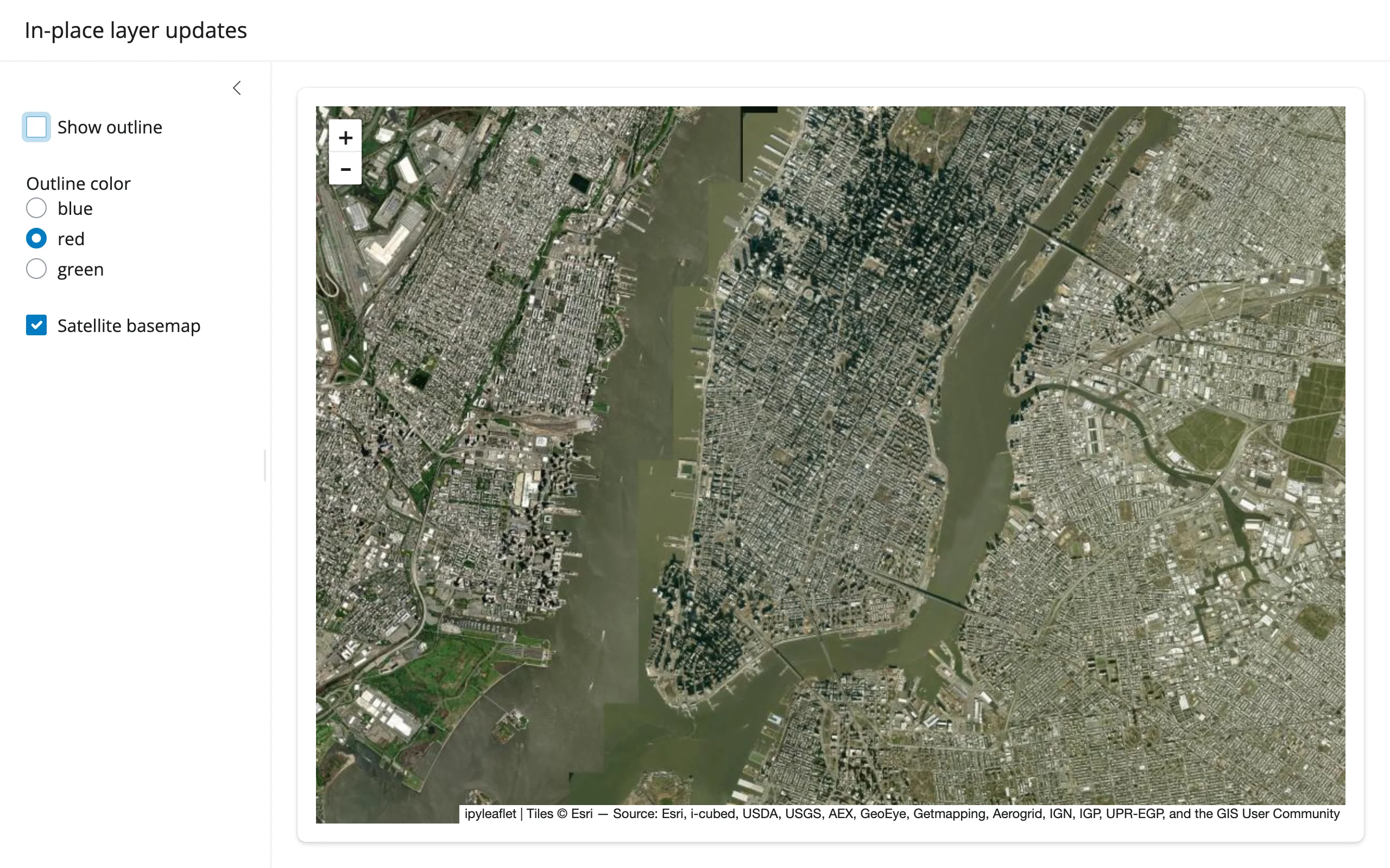
All three updates verified in Chromium: color swap, basemap swap (m.substitute()), and hiding the layer entirely via its visible trait. One easy-to-miss detail that caused a real bug while writing this guide: basemap_to_tiles() does not set base=True on its result, so if you look up “the current base layer” by layer.base after a swap and forget to set it on the replacement, the next swap’s lookup raises StopIteration – an uncaught one kills the session. Always set new.base = True on the replacement before substituting.

When to re-render instead: if the number or structure of layers changes substantially (e.g., switching datasets entirely), or you need a clean slate, re-rendering is simpler and the cost is just the widget’s own JS bundle (already cached) plus its current layer data – which can be non-trivial for many Marker widgets (see Gotchas). In-place updates still avoid the full re-render (so pan/zoom/drawn shapes survive), but don’t assume every in-place update is cheap: a visible toggle is a tiny patch (~444 bytes, measured), but a style change on a GeoJSON layer re-sends the entire feature collection with the new style baked into every feature (~1.09 MB for this example’s single-feature outline – about the same payload as just re-rendering the whole map), because ipyleaflet bakes style into each feature rather than syncing it as a separate trait. For a handful of visibility toggles, in-place updates are both less code and imperceptibly fast; for frequent style changes on data-heavy GeoJSON layers, re-rendering may cost about the same as updating in place.

Coordinating multiple views

Draw a shape, filter a table

drawn_features() returns GeoJSON; a few lines of shapely turn that into a spatial filter over any point dataset:

examples/11_linked_spatial_filter.py41 lines

import ipyleaflet as L
import plotly.express as px
from shapely.geometry import Point, shape
from shiny.express import render, ui
from shinywidgets import render_ipyleaflet

ui.page_opts(title="Draw a shape, filter the table", fillable=True)

# plotly's carshare dataset: 249 real car2go pod locations around Montreal
pods = px.data.carshare()

with ui.layout_columns(col_widths=[7, 5]):
    with ui.card():

        @render_ipyleaflet
        def map():
            m = L.Map(center=(45.52, -73.59), zoom=11)
            # rectangle={}: an empty dict disables the tool; give it a
            # (possibly empty) shapeOptions to enable it, like the other tools
            m.add(
                L.DrawControl(
                    polygon={"shapeOptions": {"color": "#2a7fff"}},
                    rectangle={"shapeOptions": {}},
                )
            )
            return m

    with ui.card(full_screen=True):
        ui.card_header("Pods inside the drawn shape(s)")

        @render.data_frame
        def inside():
            feats = map.drawn_features()  # [] until something is drawn
            if not feats:
                return pods.iloc[0:0]
            polys = [shape(f["geometry"]) for f in feats]
            mask = [
                any(poly.contains(Point(lon, lat)) for poly in polys)
                for lat, lon in zip(pods["centroid_lat"], pods["centroid_lon"])
            ]
            return render.DataGrid(pods[mask].reset_index(drop=True))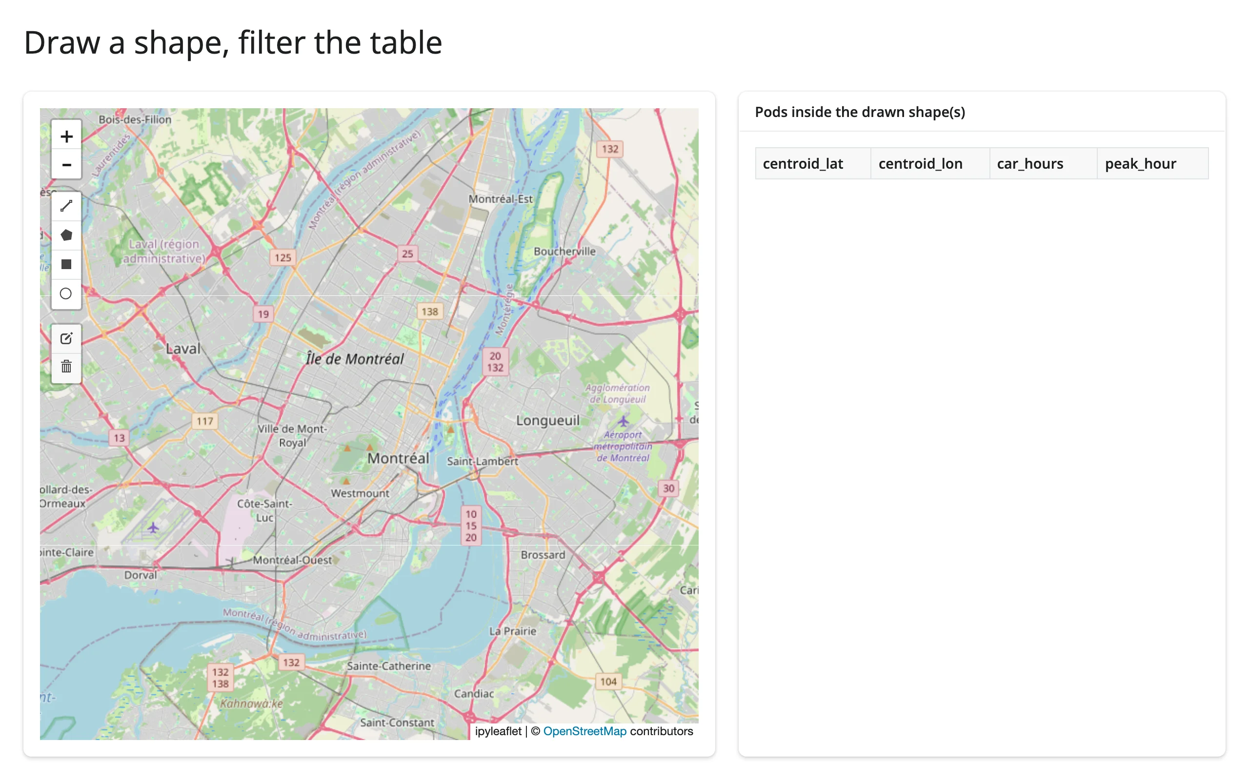

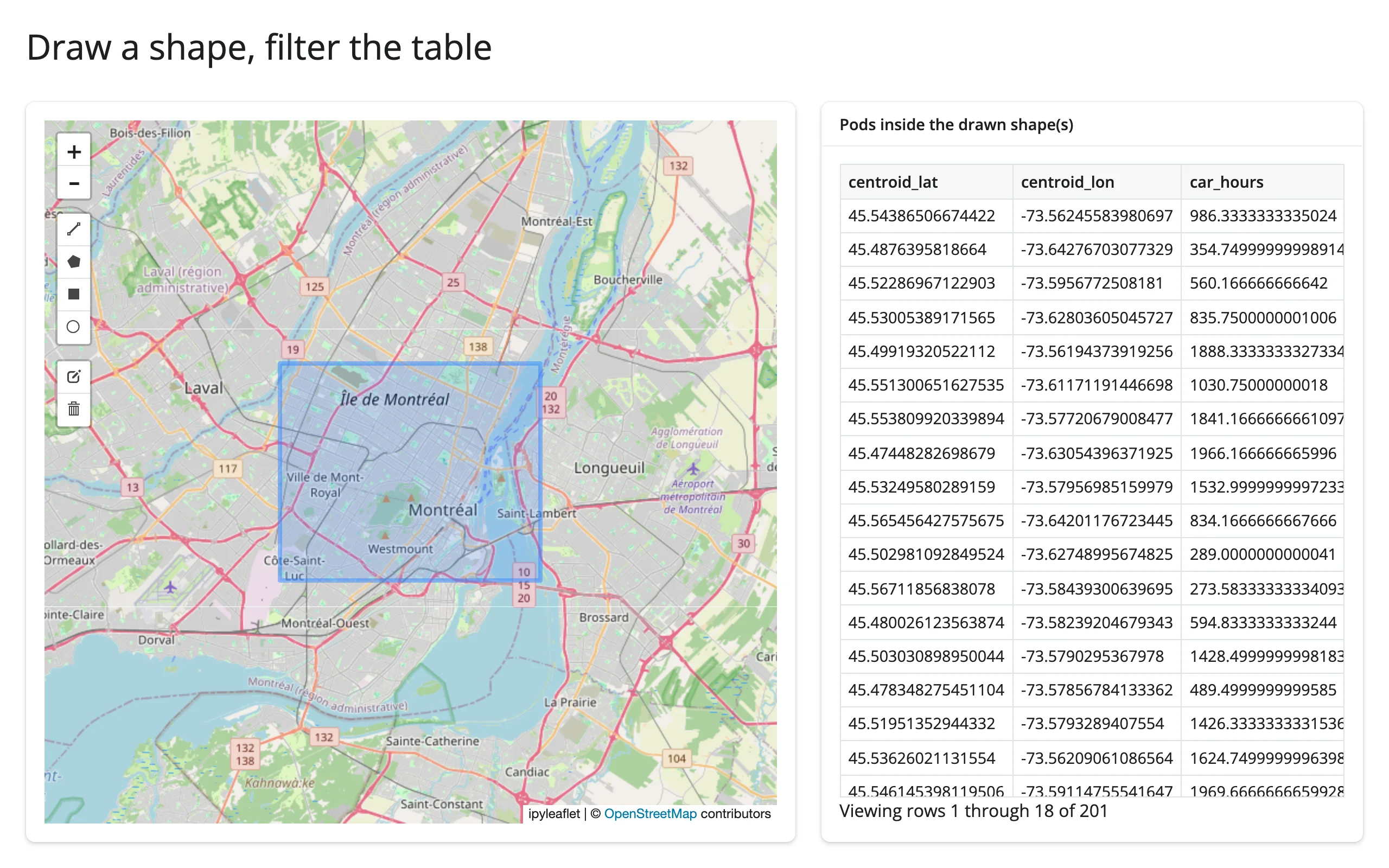
spatial filter before spatial filter after

Verified by dragging a rectangle with Playwright: the table went from empty to 201 of 249 rows, matching the drawn extent.

Map viewport, a chart of what’s visible

bounds() makes “what’s on screen” a reactive value. Pairing it with a render_plotly output (pairs with: plotly) gives a live summary of the visible subset as the user pans and zooms – no manual event wiring:

examples/12_linked_viewport_summary.py35 lines

import pandas as pd
import plotly.express as px
import ipyleaflet as L
from shiny.express import ui
from shinywidgets import render_ipyleaflet, render_plotly

ui.page_opts(title="What's in view", fillable=True)

# plotly's carshare dataset: 249 real car2go pod locations around Montreal,
# labeled with when each pod sees its heaviest use
pods = px.data.carshare()
pods["period"] = pd.cut(
    pods["peak_hour"], bins=[-1, 5, 11, 17, 23], labels=["night", "morning", "afternoon", "evening"]
)

with ui.layout_columns(col_widths=[7, 5]):
    with ui.card():

        @render_ipyleaflet
        def map():
            m = L.Map(center=(45.52, -73.59), zoom=11)
            markers = [L.Marker(location=(r.centroid_lat, r.centroid_lon)) for r in pods.itertuples()]
            m.add(L.MarkerCluster(markers=markers))
            return m

    with ui.card():
        ui.card_header("Pods in the current viewport, by peak period")

        @render_plotly
        def in_view():
            (south, west), (north, east) = map.bounds()  # pairs with: plotly
            visible = pods[pods.centroid_lat.between(south, north) & pods.centroid_lon.between(west, east)]
            counts = visible["period"].value_counts().reindex(["night", "morning", "afternoon", "evening"]).reset_index()
            counts.columns = ["period", "count"]
            return px.bar(counts, x="period", y="count")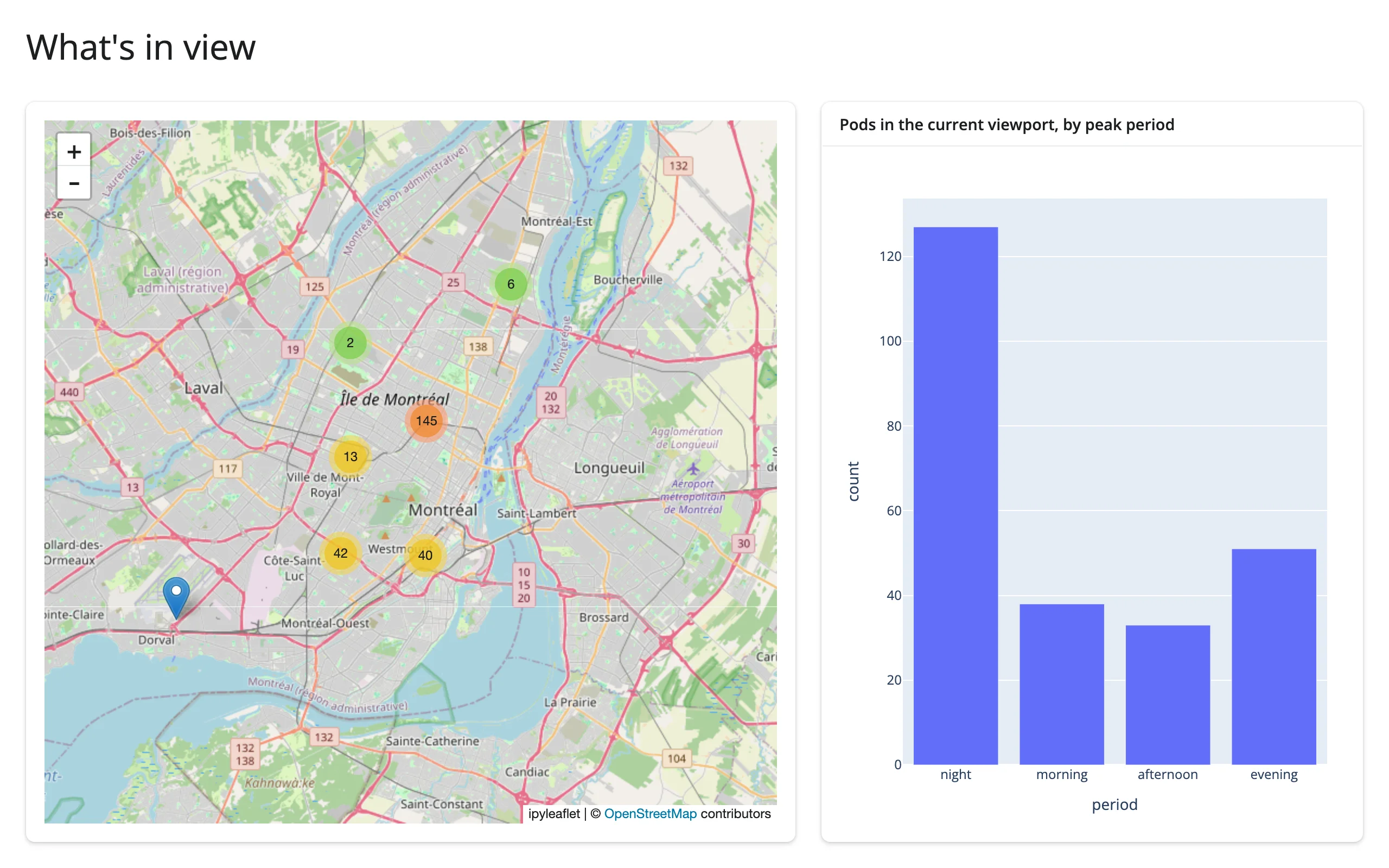

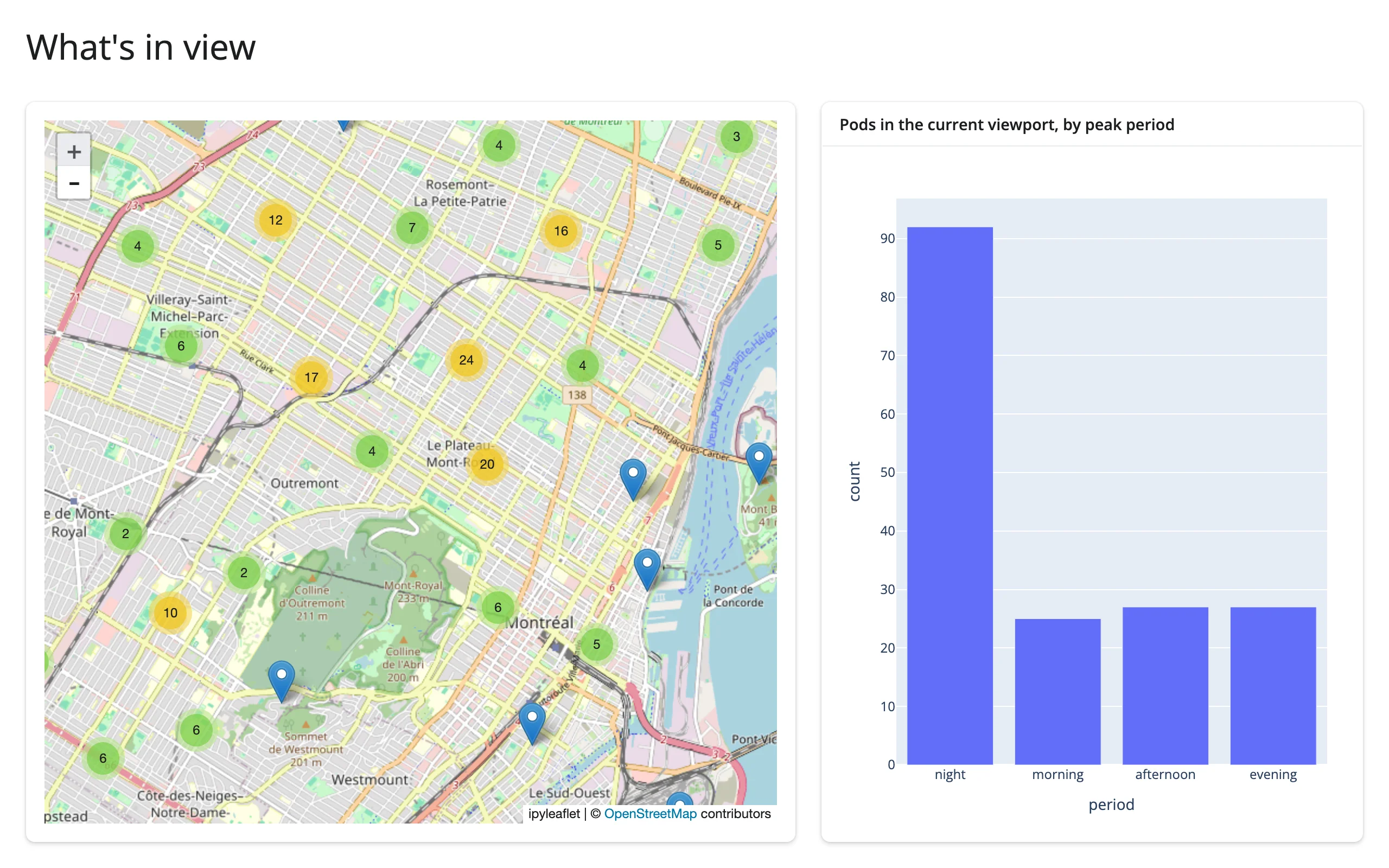
viewport before viewport after

Verified: zooming in twice dropped the chart from all 249 pods to the ~172 inside the new viewport, with the night bar shrinking proportionally more because that cluster sits further north.

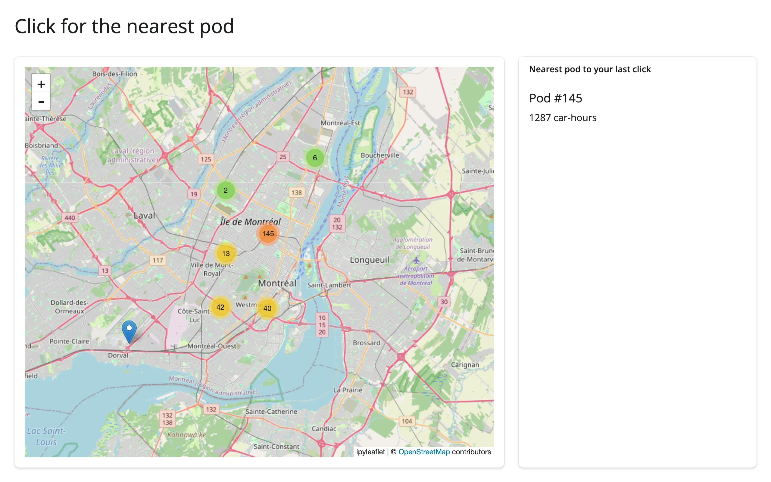
Click, find the nearest feature

clicked() plus a one-line distance calculation gives a “nearest neighbor” detail card – useful any time a dataset has too many points to label individually:

examples/13_linked_click_nearest.py32 lines

import plotly.express as px
import ipyleaflet as L
from shiny.express import render, ui
from shinywidgets import render_ipyleaflet

ui.page_opts(title="Click for the nearest pod", fillable=True)

# plotly's carshare dataset: 249 real car2go pod locations around Montreal
pods = px.data.carshare()

with ui.layout_columns(col_widths=[8, 4]):
    with ui.card():

        @render_ipyleaflet
        def map():
            m = L.Map(center=(45.52, -73.59), zoom=11)
            markers = [L.Marker(location=(r.centroid_lat, r.centroid_lon)) for r in pods.itertuples()]
            m.add(L.MarkerCluster(markers=markers))
            return m

    with ui.card():
        ui.card_header("Nearest pod to your last click")

        @render.ui
        def nearest():
            c = map.clicked()
            if c is None:
                return "Click the map."
            lat, lng = c["coordinates"]
            d2 = (pods["centroid_lat"] - lat) ** 2 + (pods["centroid_lon"] - lng) ** 2
            row = pods.loc[d2.idxmin()]
            return ui.div(ui.h5(f"Pod #{row.name}"), f"{row['car_hours']:.0f} car-hours")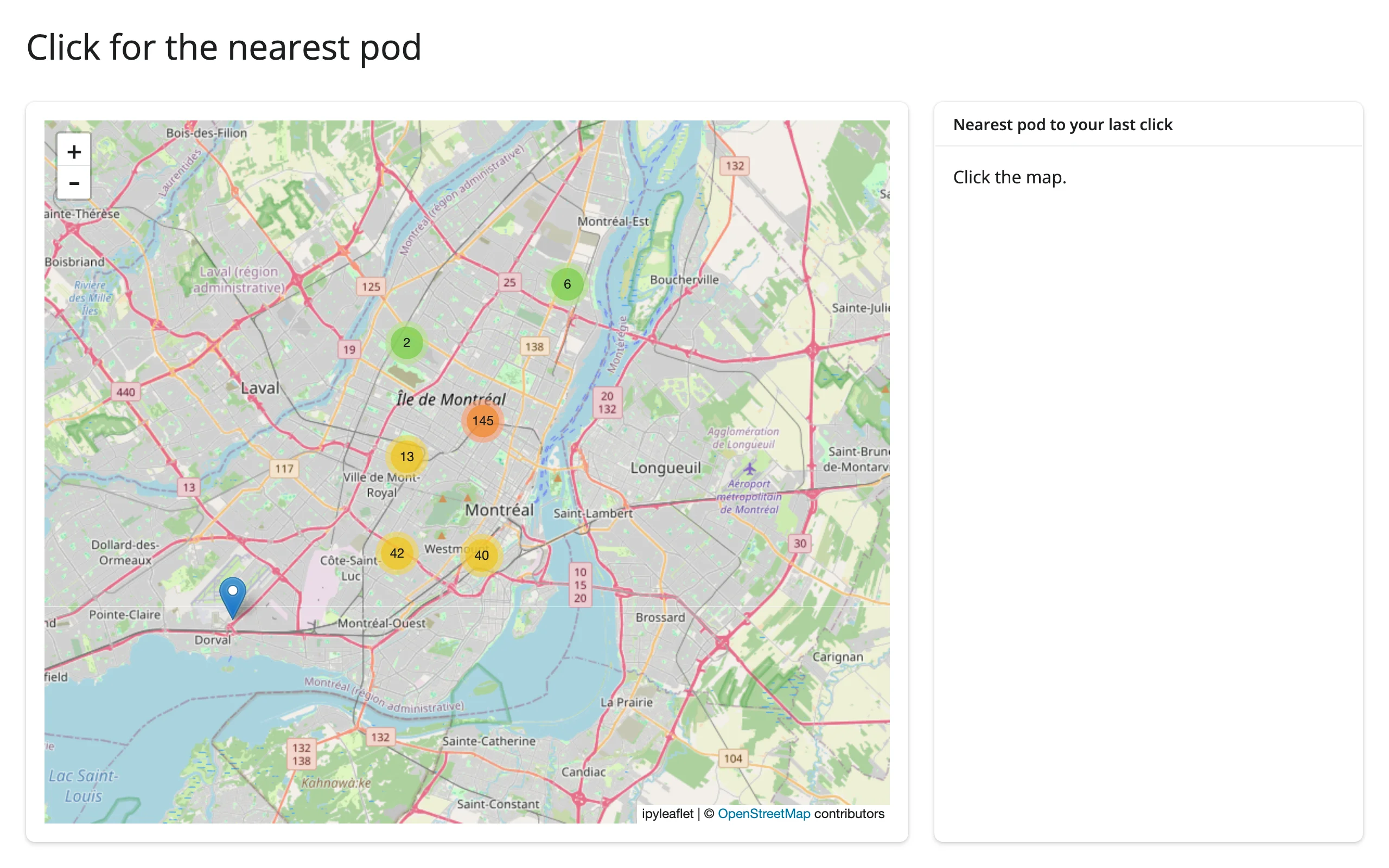

click nearest before click nearest after

Widget state updating another widget, in place

A second, smaller “overview” map stays synced to a detail map’s camera – a classic locator-map pattern. Reading center()/bounds() on the detail map and assigning to the overview’s own trait is enough; there’s no feedback loop because setting a trait to the value it already holds doesn’t re-publish:

examples/14_linked_two_maps.py35 lines

import ipyleaflet as L
from shiny import reactive
from shiny.express import ui
from shinywidgets import render_ipyleaflet

ui.page_opts(title="Overview map stays in sync", fillable=True)

with ui.layout_columns(col_widths=[8, 4]):
    with ui.card():

        @render_ipyleaflet
        def main():
            return L.Map(center=(40.73, -73.99), zoom=14)

    with ui.card():

        @render_ipyleaflet
        def overview():
            m = L.Map(center=(40.73, -73.99), zoom=10)
            m.add(L.Rectangle(bounds=((40.72, -74.0), (40.74, -73.98)), name="extent"))
            return m


# The overview map never re-renders: panning or zooming the main map just
# moves its center and resizes its rectangle, so the overview keeps its own
# zoom level and any layers a user added to it.
@reactive.effect
def _sync_overview_center():
    overview.widget.center = main.center()


@reactive.effect
def _sync_extent_rectangle():
    extent = next(lyr for lyr in overview.widget.layers if lyr.name == "extent")
    extent.bounds = main.bounds()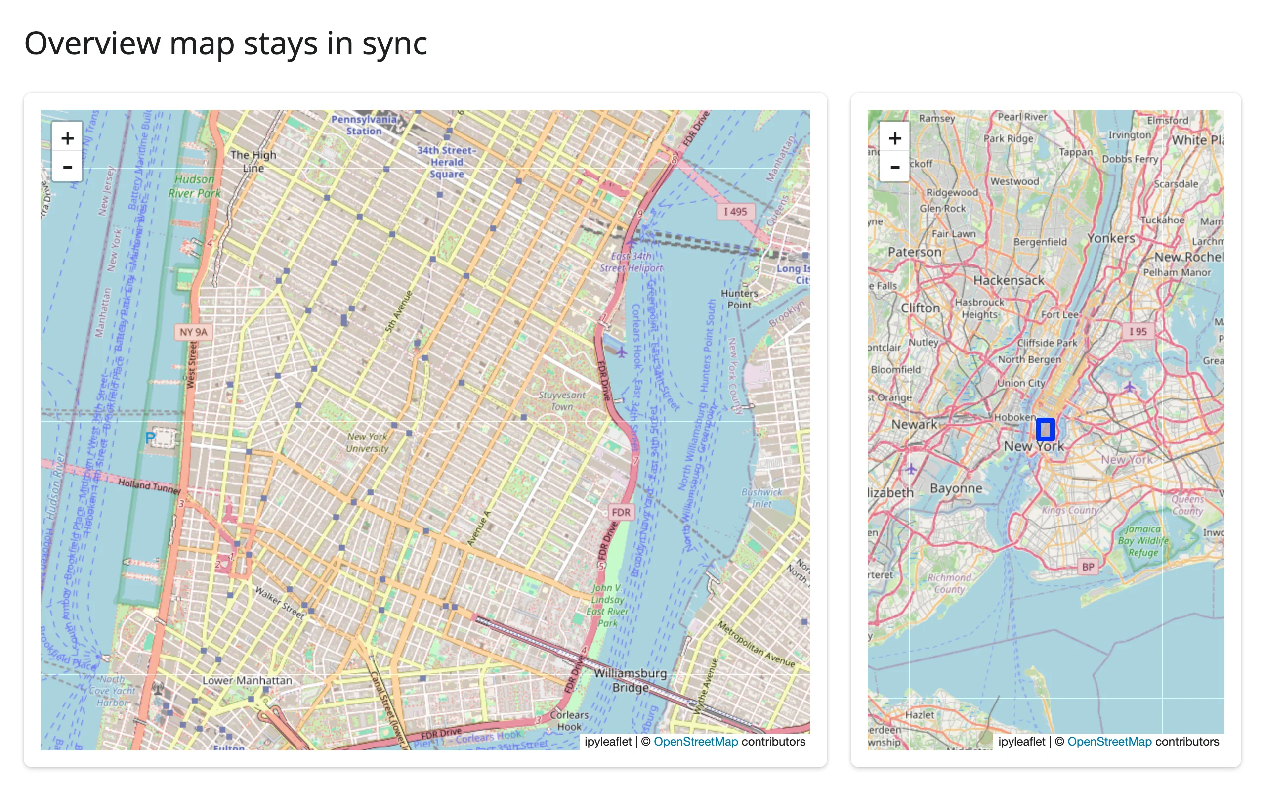

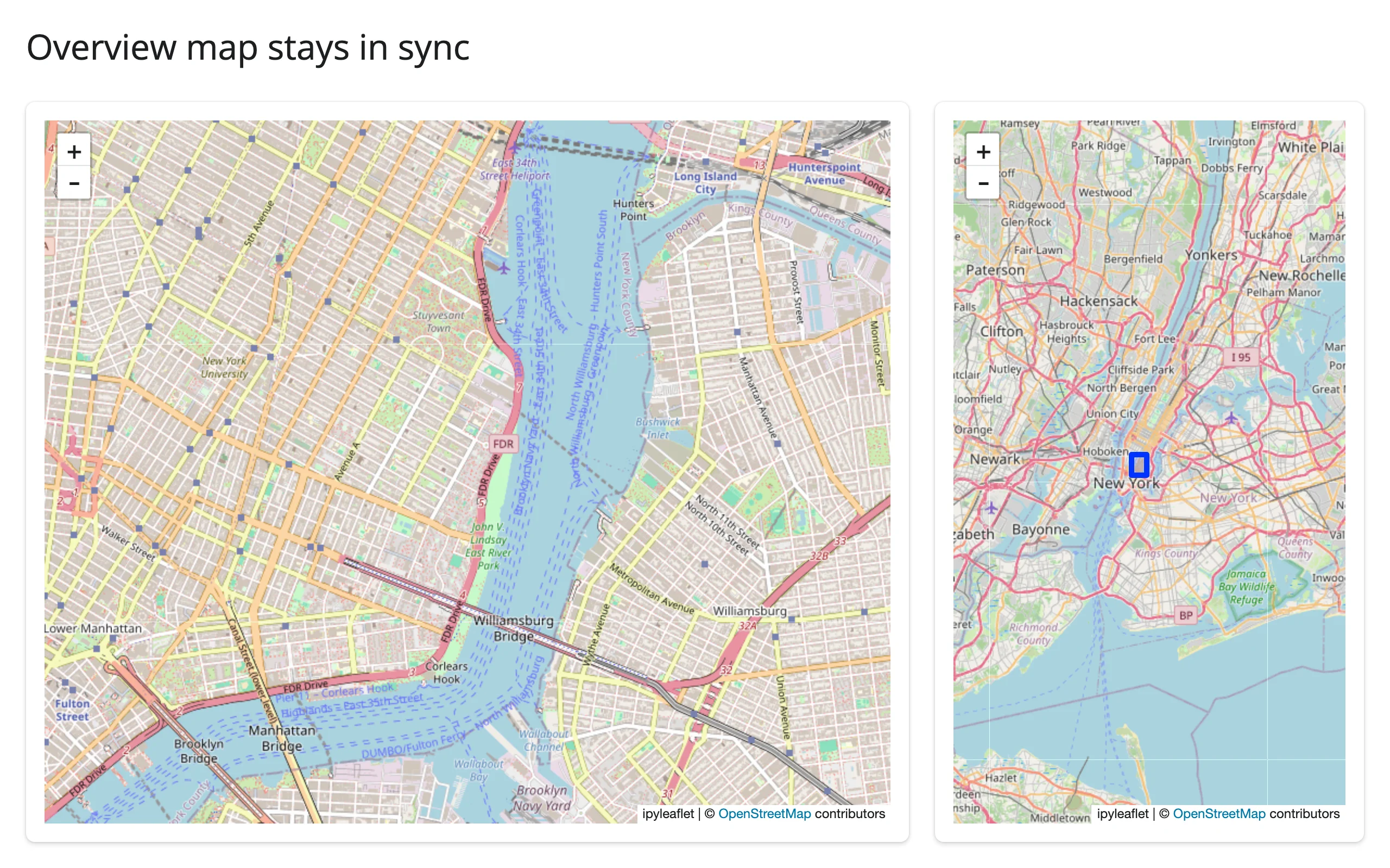
Verified by dragging the main map: the overview’s center and its extent rectangle both followed, while the overview kept its own, more zoomed-out, view.

Large data

ipyleaflet has no large-data mode of its own: every marker and GeoJSON feature you add is sent to the browser in full and drawn in the DOM/SVG, which is why marker clustering only helps into the low thousands of points, not beyond. Its basemap tiles are the exception – raster tile layers only ever load the tiles the current viewport needs, “only send what’s visible,” but that applies to the basemap, not your data. For a real point cloud (tens of thousands of rows or more), hand the same data to lonboard instead, which draws it with the GPU rather than the DOM – see this guide’s introduction for the comparison. For local raster files, pair ipyleaflet with localtileserver, which gives your own raster data the same only-send-what’s-visible treatment the basemap gets. See the Large data & performance article for how these approaches compare in general.

Layout and sizing

The map fills its container in a filling layout (card, fillable=True page) unless it has its own height, either via output_widget(height=...) or Layout(height=...) on the Map. A subclass’s own default height (e.g., leafmap’s 600px) is treated as unset – see the leafmap guide for that renderer’s specifics.
Use output_widget(height="300px") (or @render_ipyleaflet(height=...) in Express) for a fixed size. output_widget(height="auto")/"fit-content" are handled correctly (an older build of this renderer briefly turned those into a 0-height map; that’s fixed on current main).
full_screen=True cards work as expected; Leaflet resizes to fill the expanded card.
A map in a hidden tab initializes at the correct size once the tab is shown (Shiny suspends the output while hidden), and resizing while hidden is tracked correctly.

Gotchas and limitations

Multiple base=True layers all render until the user interacts. ipyleaflet doesn’t pick one for you up front: every base tile layer you .add() stays visible=True, so with several of them, whichever was added last ends up on top and is what’s actually shown – regardless of which radio button the LayersControl marks as selected. The fix (used in the basemaps example above) is to re-add your intended default layer last. This is reproducible on current main; we haven’t checked whether it’s ipyleaflet-the-Python-package or jupyter-leaflet-the-frontend’s doing.
rectangle={}/circle={} on DrawControl silently disables the tool. The traits default to {}, which looks “on” from Python, but the frontend only enables a tool when its options dict is non-empty (the other tools default to {"shapeOptions": {}}, which has one key). Pass {"shapeOptions": {}} explicitly to enable rectangle or circle drawing.
basemap_to_tiles() doesn’t set base=True. If your own code looks up “the current base layer” by layer.base (as the in-place basemap swap above does), the replacement needs new.base = True set explicitly, or the next lookup raises StopIteration – uncaught, that kills the session.
A double-click publishes clicked() once, not twice. The browser sends two native click events plus a dblclick for a double-click; both clicks land on the same coordinate, and clicked() dedupes identical consecutive values like any other input, so only one update reaches Python. See the clicked() section above.
Clicks on a layer also reach the map’s clicked(). Leaflet events bubble, so clicking a GeoJSON feature fires both that layer’s own on_click and the map’s clicked(). Not independently re-verified for this guide (carried over from the prior evaluation report), but it follows directly from Leaflet’s event model.
Prefer one GeoJSON layer over many Marker widgets for large point counts. Each Marker is its own ipywidgets model with its own comm traffic; a single GeoJSON layer with point_style/style_callback is far cheaper to construct and re-send, and is what the choropleth and “coordinating multiple views” examples above use for anything beyond a few hundred points.
Map controls can look transparent outside JupyterLab. jupyter-leaflet’s CSS reads --jp-* theme variables with no fallback; those variables don’t exist until some other Jupyter-widgets control has loaded CSS. In this guide’s screenshots the zoom buttons and draw toolbar render with solid backgrounds, so this does not currently reproduce on main – it may already be mitigated, or may depend on which other widgets are on the page. Flagging as a known upstream wart rather than a confirmed current bug.

Gallery candidates

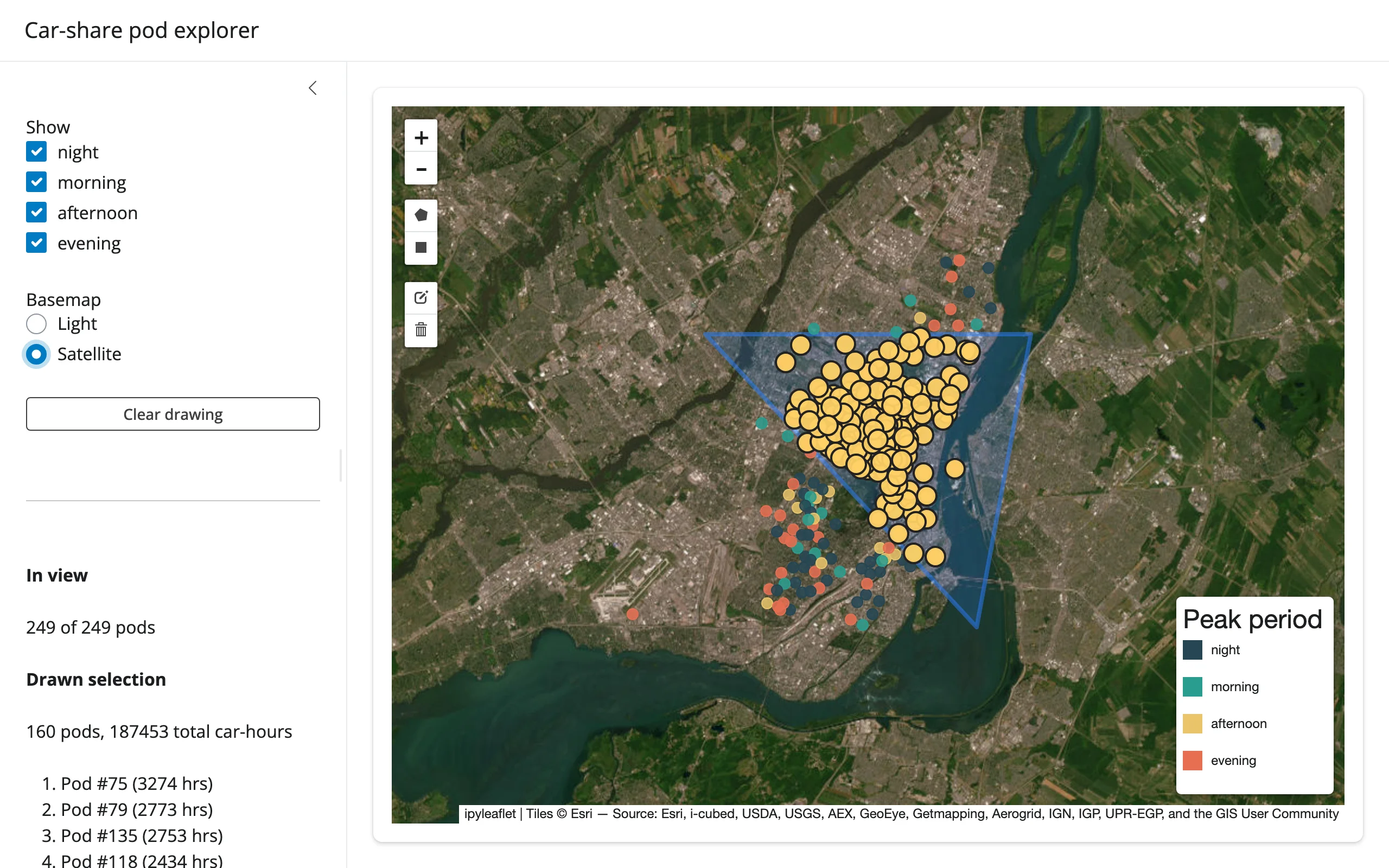
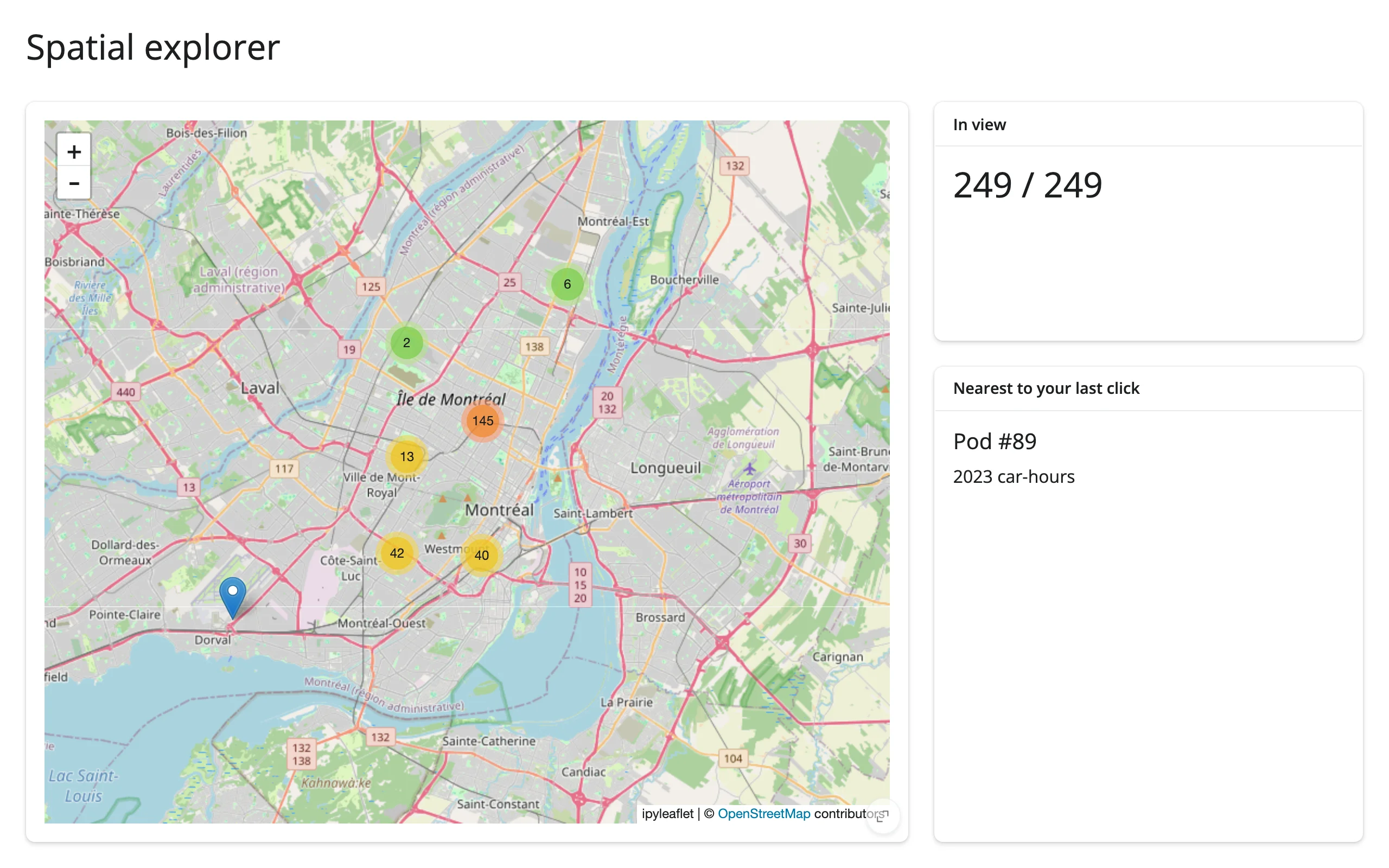
gallery/template_spatial_explorer.py (template, ~55 lines) – a clean starting point for any point dataset: clustered markers, a live “N in view” count from bounds(), and a click-to-detail card from clicked().

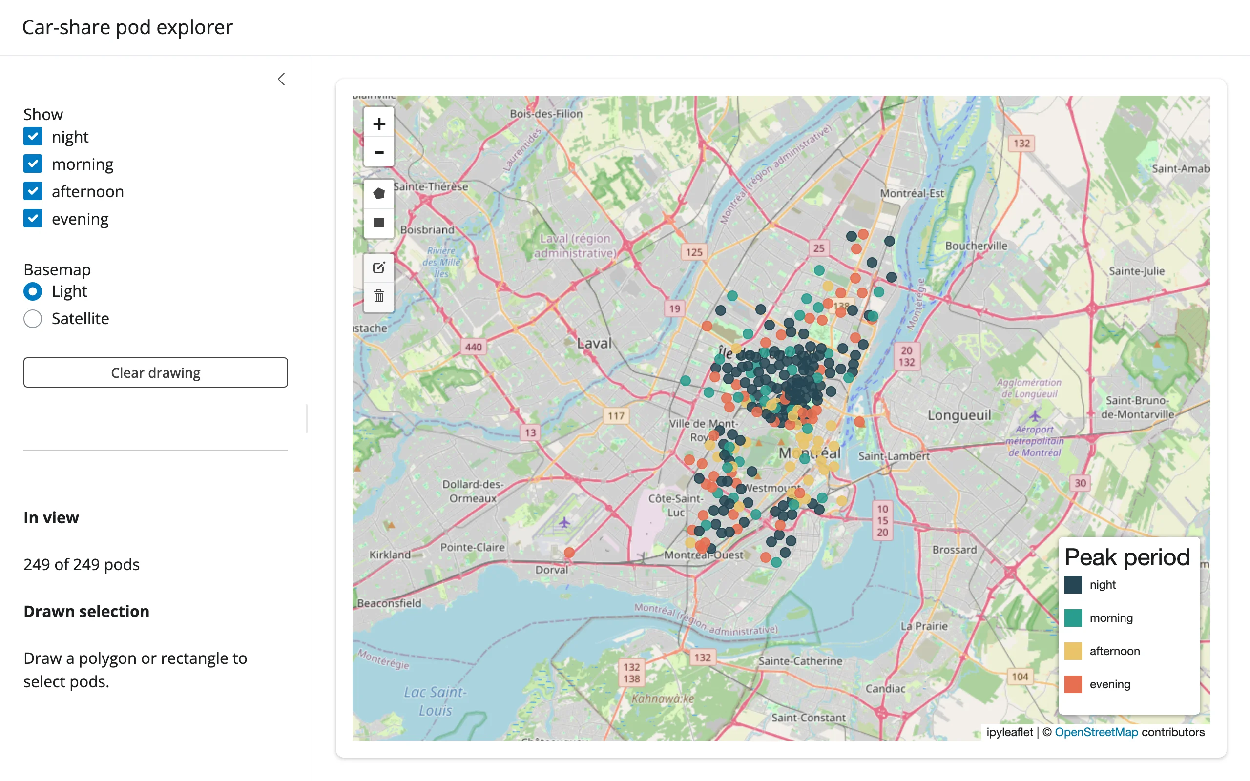
gallery/showcase_carshare_explorer.py (showcase, ~155 lines) – draw a shape and get the count, total usage, and busiest-pod shortlist inside it, highlighted on the map without re-rendering; filter by time-of-day and swap basemaps, both in place. Uses drawn_features() and bounds().

showcase before showcase after

Learn more

ipyleaflet documentation
Leaflet.js (the underlying JS library) and Leaflet.draw (the drawing toolbar)
shinywidgets.reactive_read for reading any widget trait
Related guides: leafmap (same accessors, more basemaps and tools), lonboard (GPU-accelerated large point/polygon layers), maplibre (vector tiles, globe), localtileserver (local raster tiles)