bqplot
bqplot is a 2D plotting library built by Bloomberg on the Grammar of Graphics, the same idea behind ggplot2 and Vega-Lite: a plot is scales (data-to-pixel mappings), marks (what gets drawn), and axes (the scales rendered as guides). Unlike most Python plotting libraries, bqplot’s plots are interactive widgets from the ground up – every mark, scale, and axis is a stateful object with traits, and bqplot ships a set of “interaction” widgets (brush, lasso, index selectors, pan/zoom) that write back to those traits as the user drags. That makes bqplot one of the few libraries where turning a chart into an input is the normal way to use it, not a bolt-on feature.
@render_bqplot renders a bqplot.Figure (including one built with the bqplot.pyplot shortcut interface) as a Shiny output, with no coercion step – you build the figure exactly as you would in a notebook, and the renderer handles sizing (filling its card by default), theme variables so plots and tooltips follow Shiny’s light/dark mode, and the bookkeeping needed for bqplot’s built-in toolbar (pan/zoom, reset, save-as-PNG) to work without a Jupyter kernel. Three accessors – selected(), selected_rows() (the selected rows of a data frame), and brush() – expose what the user has selected or brushed as plain Python values you read reactively, and because mutating a mark’s data in place tweens it smoothly (set Figure.animation_duration once), bqplot is also the strongest “update a plot without re-rendering it” story in the shinywidgets roster.
Reach for bqplot when you want a plot that doubles as a multi-point input (brush-to-filter, lasso-to-select, click-and-drag) or when you want data updates to animate smoothly in place, as in a scrubber or a live feed. For one-shot statistical charts with a high-level API, plotly or altair usually get you there faster; for exploring a single large table, pair bqplot with itables or reactable rather than building the table in bqplot.
Installation
pip install 'shinywidgets[bqplot]'Quick start
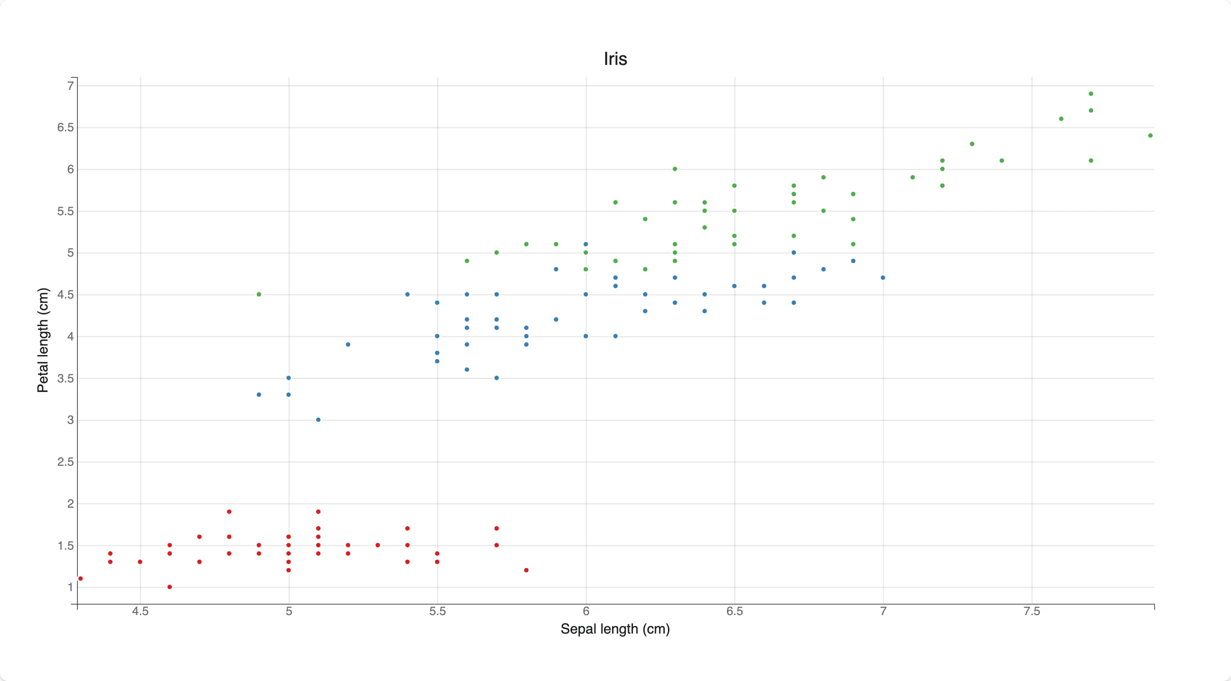
A figure is scales, a mark built on those scales, and axes that render the scales. Nothing here is bqplot specific to Shiny – @render_bqplot just displays the Figure you return and keeps it sized to its card.
# bqplot quick start: a scatter plot colored by species
import bqplot
import plotly.express as px
from shiny.express import ui
from shinywidgets import render_bqplot

ui.page_opts(title="bqplot quick start", fillable=True)

iris = px.data.iris()

with ui.card(full_screen=True):

    @render_bqplot
    def plot():
        x_sc, y_sc = bqplot.LinearScale(), bqplot.LinearScale()
        c_sc = bqplot.OrdinalColorScale(scheme="Set1")
        scatter = bqplot.Scatter(
            x=iris["sepal_length"],
            y=iris["petal_length"],
            color=iris["species"],
            scales={"x": x_sc, "y": y_sc, "color": c_sc},
            default_size=28,
            stroke="white",
        )
        return bqplot.Figure(
            marks=[scatter],
            axes=[
                bqplot.Axis(scale=x_sc, label="Sepal length (cm)"),
                bqplot.Axis(
                    scale=y_sc, orientation="vertical", label="Petal length (cm)"
                ),
            ],
            title="Iris",
        )
What you can build
The grammar: scales, marks, axes
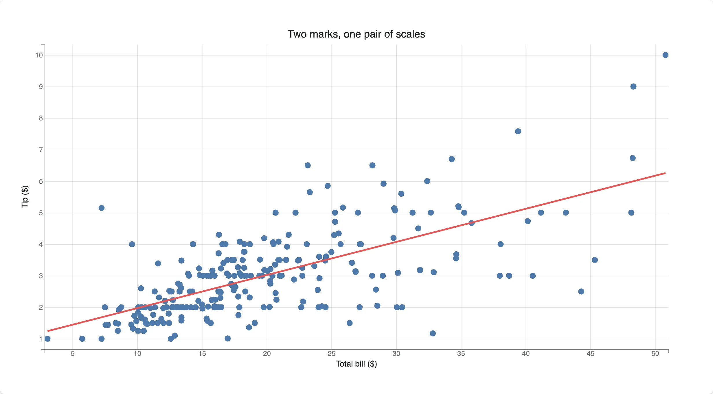
Scales are shared, not owned by a mark, so two marks on the same x_sc/y_sc always line up – here a Scatter and a fitted Lines mark share one coordinate system.
# The grammar: scales map data to pixels, marks draw on top of scales, axes
# render the scales. Two marks sharing one pair of scales stay aligned.
import bqplot
import numpy as np
import plotly.express as px
from shiny.express import ui
from shinywidgets import render_bqplot

ui.page_opts(title="bqplot grammar", fillable=True)

tips = px.data.tips()

with ui.card(full_screen=True):

    @render_bqplot
    def plot():
        x_sc, y_sc = bqplot.LinearScale(), bqplot.LinearScale()

        points = bqplot.Scatter(
            x=tips["total_bill"],
            y=tips["tip"],
            scales={"x": x_sc, "y": y_sc},
            colors=["#4c78a8"],
            default_opacities=[0.6],
        )

        # A second mark on the *same* scales: a least-squares fit line
        slope, intercept = np.polyfit(tips["total_bill"], tips["tip"], 1)
        xs = np.array([tips["total_bill"].min(), tips["total_bill"].max()])
        fit = bqplot.Lines(
            x=xs,
            y=slope * xs + intercept,
            scales={"x": x_sc, "y": y_sc},
            colors=["#e45756"],
            stroke_width=3,
        )

        return bqplot.Figure(
            marks=[points, fit],
            axes=[
                bqplot.Axis(scale=x_sc, label="Total bill ($)"),
                bqplot.Axis(scale=y_sc, orientation="vertical", label="Tip ($)"),
            ],
            title="Two marks, one pair of scales",
        )
bqplot.pyplot: a matplotlib-like shortcut
bqplot.pyplot (usually imported as bplt) builds the same object model without naming scales explicitly – bplt.scatter(), bplt.plot(), bplt.hist() and friends plot onto an implicit “current figure.” It’s faster to write but has one sharp edge in Shiny: see Gotchas.
# The same plot through bqplot.pyplot's matplotlib-like shortcuts. Always
# call bplt.figure() first and return its result -- see "Gotchas" for why.
import bqplot.pyplot as bplt
import numpy as np
import plotly.express as px
from shiny.express import ui
from shinywidgets import render_bqplot

ui.page_opts(title="bqplot.pyplot", fillable=True)

tips = px.data.tips()

with ui.card(full_screen=True):

    @render_bqplot
    def plot():
        fig = bplt.figure(title="Two marks, one pair of scales")
        bplt.scatter(
            tips["total_bill"],
            tips["tip"],
            colors=["#4c78a8"],
            default_opacities=[0.6],
        )
        slope, intercept = np.polyfit(tips["total_bill"], tips["tip"], 1)
        xs = np.array([tips["total_bill"].min(), tips["total_bill"].max()])
        bplt.plot(xs, slope * xs + intercept, colors=["#e45756"], stroke_width=3)
        bplt.xlabel("Total bill ($)")
        bplt.ylabel("Tip ($)")
        return fig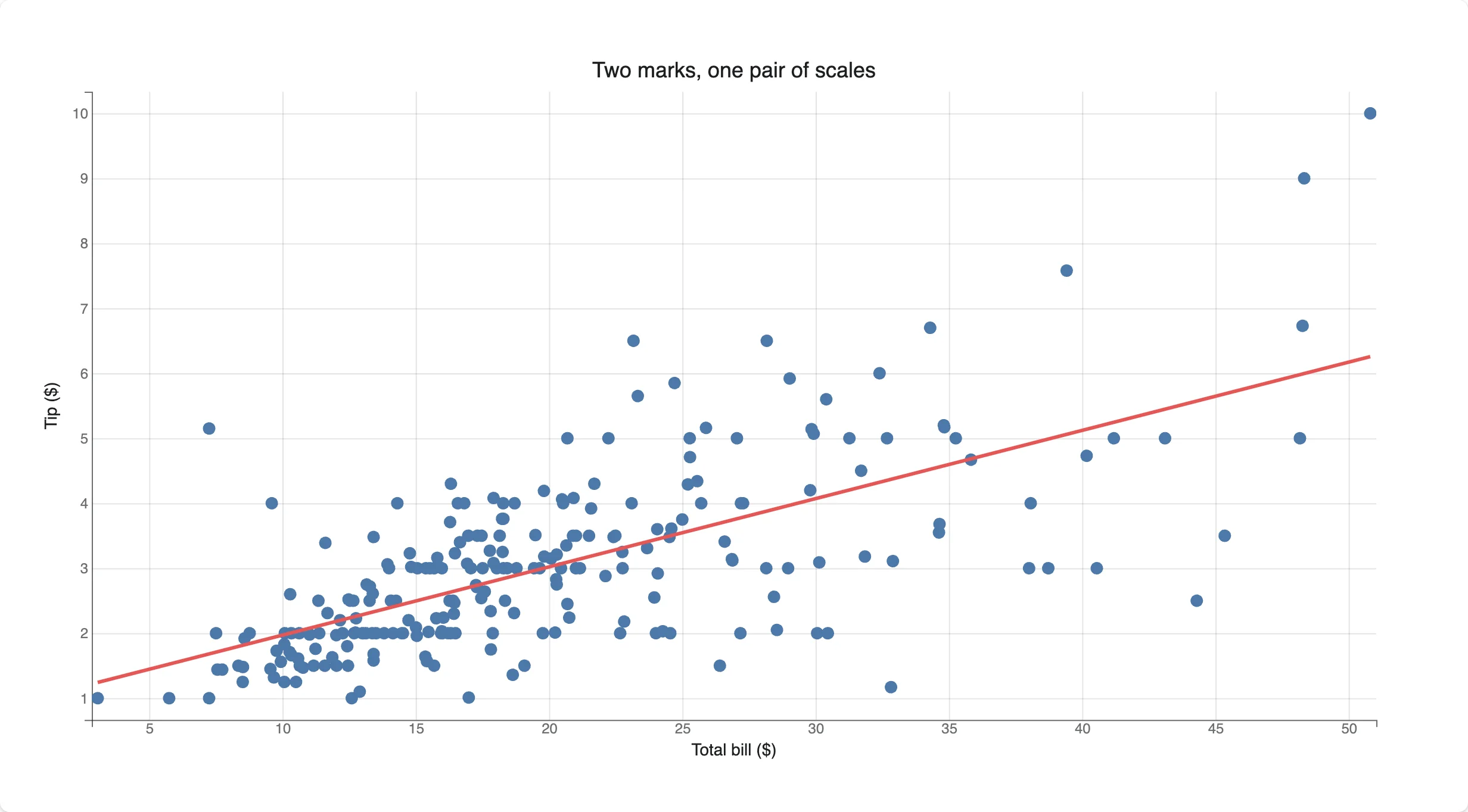
Pixel-for-pixel identical to the object-model version above – bqplot.pyplot is sugar over the same Figure.
Drag the data
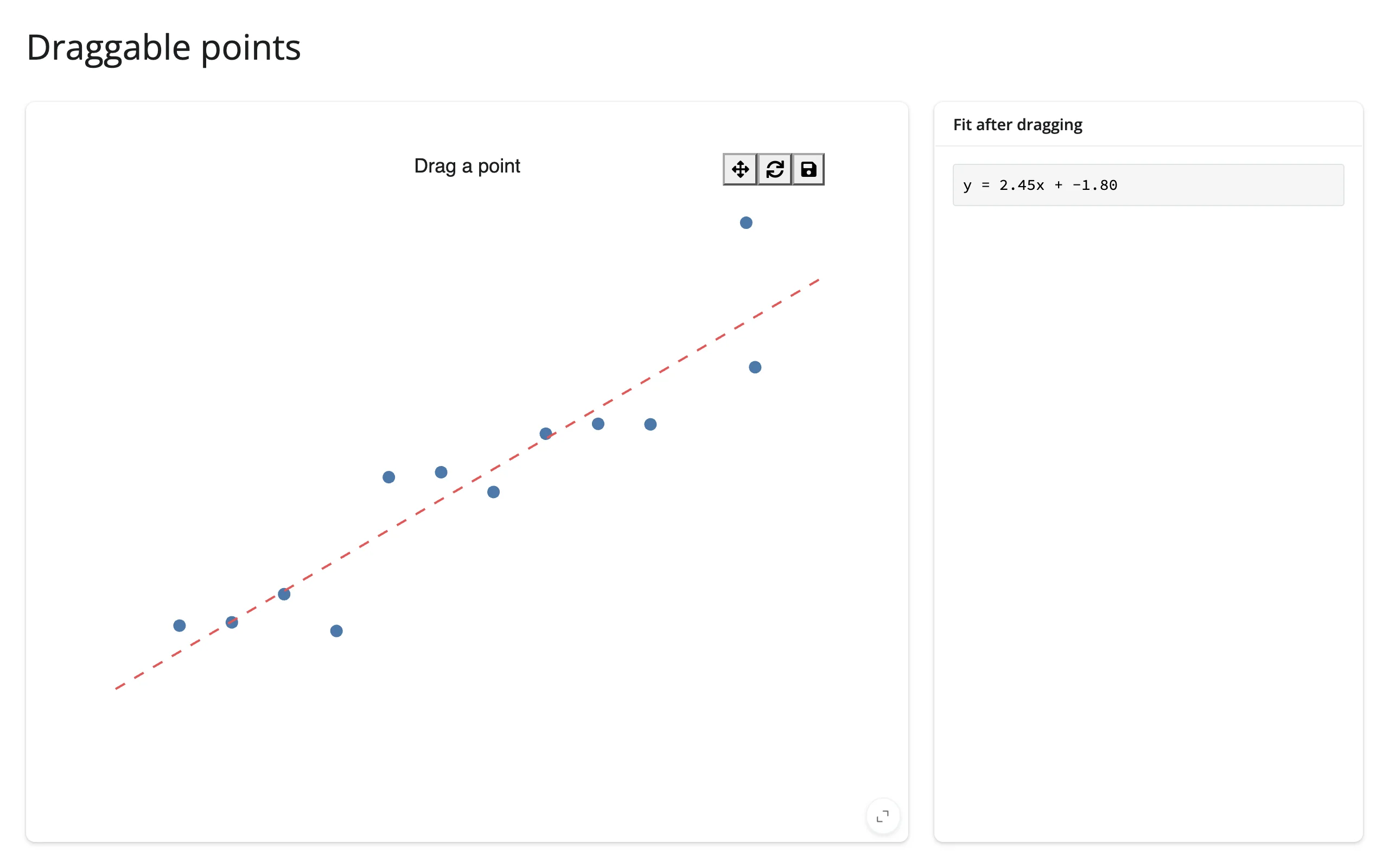
Set enable_move=True on a Scatter and users can pull points around with the mouse; the new x/y land back in Python once the drag ends (update_on_move=True streams them continuously instead). Combined with reactive_read, a dragged point can refit a regression line live.
# Draggable marks: enable_move lets users pull points around. x/y land back
# in Python once the drag ends (set update_on_move=True to stream mid-drag).
import bqplot
import numpy as np
from shiny.express import render, ui
from shinywidgets import reactive_read, render_bqplot

ui.page_opts(title="Draggable points", fillable=True)

rng = np.random.default_rng(2)
x0 = np.linspace(1, 10, 12)
y0 = 2 * x0 + rng.normal(0, 2, 12)

with ui.layout_columns(col_widths=[8, 4]):
    with ui.card(full_screen=True):

        @render_bqplot
        def plot():
            x_sc = bqplot.LinearScale(min=0, max=11)
            y_sc = bqplot.LinearScale(min=-5, max=30)
            points = bqplot.Scatter(
                x=x0.copy(),
                y=y0.copy(),
                scales={"x": x_sc, "y": y_sc},
                colors=["#4c78a8"],
                default_size=80,
                enable_move=True,
            )
            fit = bqplot.Lines(
                x=[0, 11],
                y=[0, 22],
                scales={"x": x_sc, "y": y_sc},
                colors=["#e45756"],
                stroke_width=2,
                line_style="dashed",
            )
            return bqplot.Figure(marks=[points, fit], title="Drag a point")

    with ui.card():
        ui.card_header("Fit after dragging")

        @render.code
        def fit_summary():
            points = plot.widget.marks[0]
            x = reactive_read(points, "x")
            y = reactive_read(points, "y")
            slope, intercept = np.polyfit(x, y, 1)

            # In-place update: mutate the existing Lines mark rather than
            # re-rendering the figure, so the drag the user just made stays put
            fit = plot.widget.marks[1]
            xs = np.array([0.0, 11.0])
            fit.x, fit.y = xs, slope * xs + intercept

            return f"y = {slope:.2f}x + {intercept:.2f}"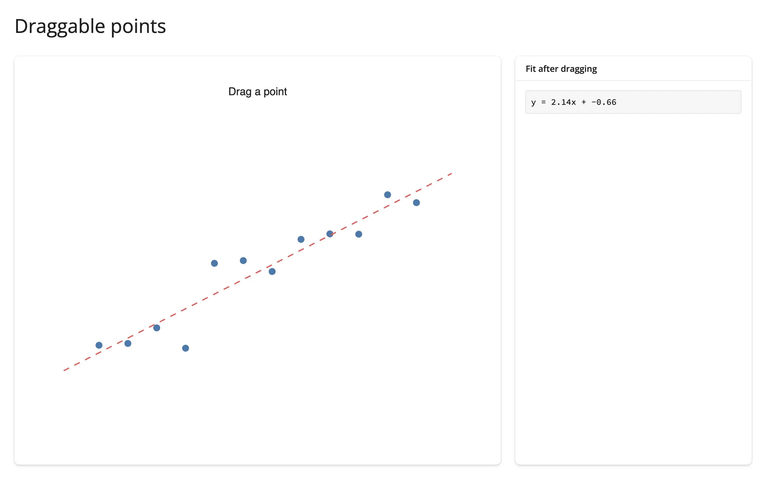
Smooth, animated updates – bqplot’s signature move
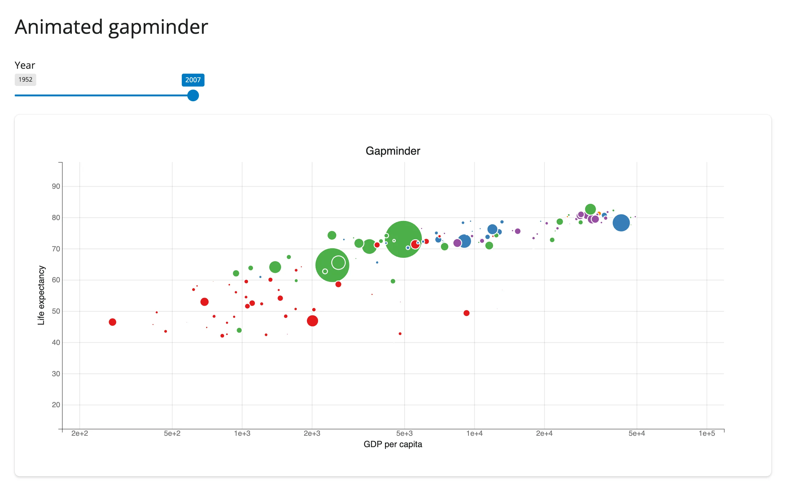
Set Figure.animation_duration once; after that, any trait change to a mark’s data tweens to its new value instead of snapping. This is the classic Hans Rosling “bubble chart over time” demo, and it is genuinely different from re-rendering: the dots glide between years rather than disappearing and reappearing.
# bqplot's signature move: set Figure.animation_duration once, then mutate a
# mark's data in an effect. bqplot tweens the points to their new positions
# instead of redrawing, so the slider feels like it's scrubbing through time.
import bqplot
import plotly.express as px
from shiny import reactive
from shiny.express import input, render, ui
from shinywidgets import render_bqplot

ui.page_opts(title="Animated gapminder", fillable=True)

gap = px.data.gapminder()
years = sorted(int(y) for y in gap["year"].unique())
continents = sorted(gap["continent"].unique())

ui.input_slider("year", "Year", min(years), max(years), min(years), step=5, sep="")

with ui.card(full_screen=True):

    @render_bqplot
    def bubbles():
        x_sc = bqplot.LogScale(min=200, max=1e5)
        y_sc = bqplot.LinearScale(min=20, max=90)
        c_sc = bqplot.OrdinalColorScale(domain=continents, scheme="Set1")
        size_sc = bqplot.LinearScale(min=0.0, max=float(gap["pop"].max()))

        points = bqplot.Scatter(
            scales={"x": x_sc, "y": y_sc, "color": c_sc, "size": size_sc},
            default_size=3000,
            default_opacities=[0.7],
            stroke="white",
        )
        fig = bqplot.Figure(
            marks=[points],
            axes=[
                bqplot.Axis(scale=x_sc, label="GDP per capita"),
                bqplot.Axis(scale=y_sc, orientation="vertical", label="Life expectancy"),
            ],
            title="Gapminder",
            animation_duration=750,
        )
        return fig

    @reactive.effect
    def _update_year():
        year_data = gap[gap["year"] == input.year()]
        points = bubbles.widget.marks[0]
        # Setting several traits inside one hold_sync() batches them into a
        # single update message, so the browser doesn't tween x, then y, then
        # size as three separate steps
        with points.hold_sync():
            points.x = year_data["gdpPercap"].to_numpy()
            points.y = year_data["lifeExp"].to_numpy()
            points.color = year_data["continent"].to_numpy()
            points.size = year_data["pop"].to_numpy()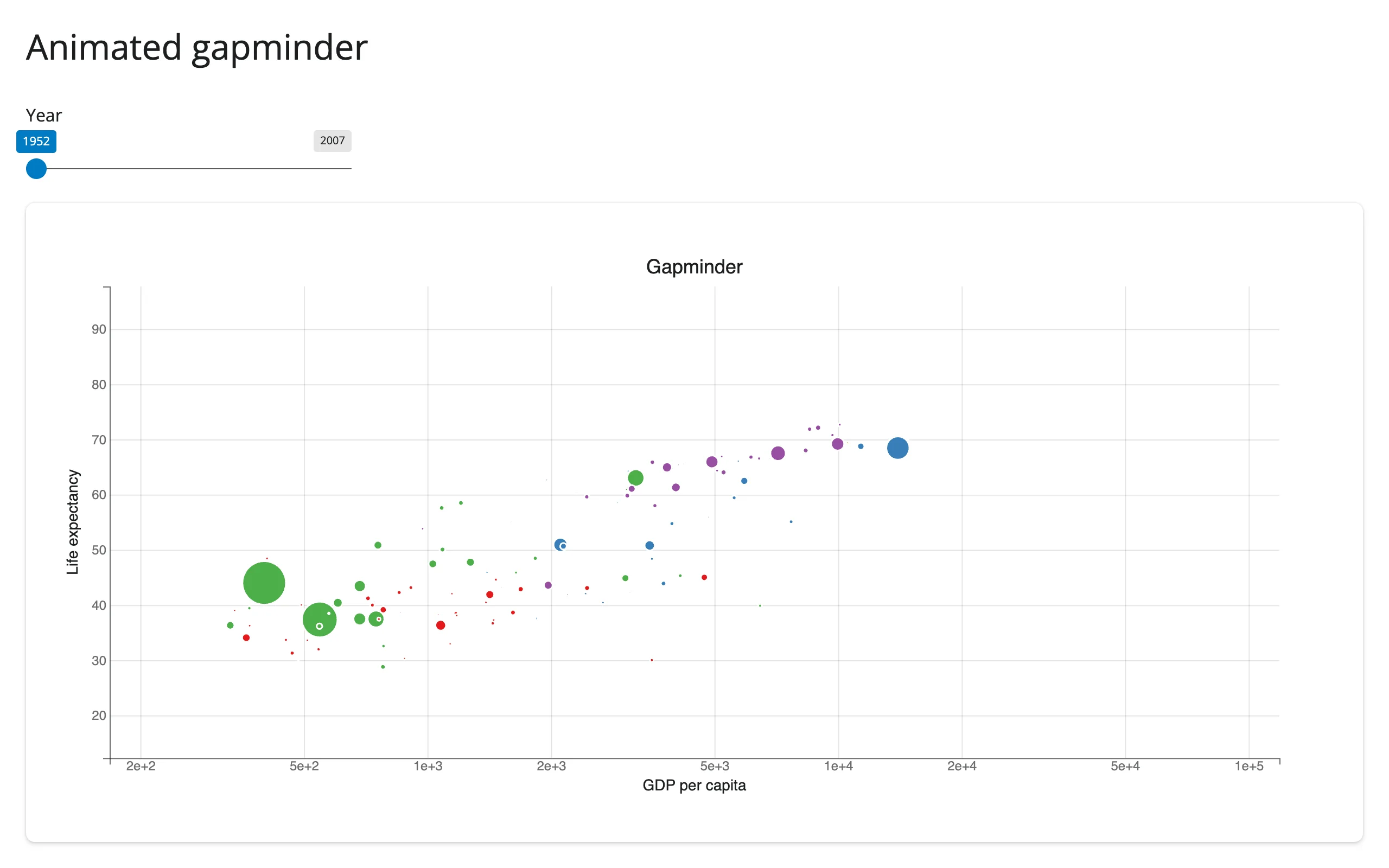
Note default_size: when a mark has a size scale, default_size is the maximum marker area in pixels, not a per-point constant – set it too low (the bqplot default is 64) and bubbles with meaningful population values can render invisibly small.
The built-in toolbar works
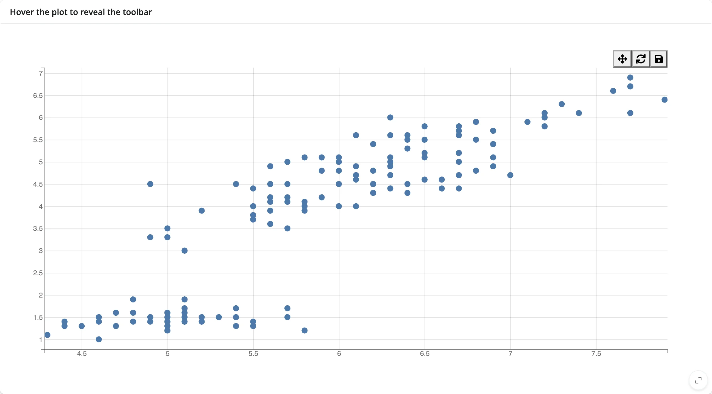
bqplot figures can carry a toolbar (display_toolbar=True, the default in some constructors) with pan/zoom, reset, and save-as-PNG. The pan/zoom button creates a bqplot.interacts.PanZoom widget from the browser, which historically needed a Jupyter kernel to open its comm; shinywidgets now opens that comm on demand, so the toolbar works out of the box, including reset (which closes the PanZoom model cleanly) and PNG export.
# The figure's built-in toolbar (pan/zoom, reset, save as PNG) needs its own
# widgets in the browser. shinywidgets opens their Python counterparts on
# demand, so the buttons work without any extra code.
import bqplot
import plotly.express as px
from shiny.express import ui
from shinywidgets import render_bqplot

ui.page_opts(title="Toolbar", fillable=True)

iris = px.data.iris()

with ui.card(full_screen=True):
    ui.card_header("Hover the plot to reveal the toolbar")

    @render_bqplot
    def plot():
        x_sc, y_sc = bqplot.LinearScale(), bqplot.LinearScale()
        scatter = bqplot.Scatter(
            x=iris["sepal_length"],
            y=iris["petal_length"],
            scales={"x": x_sc, "y": y_sc},
            colors=["#4c78a8"],
        )
        return bqplot.Figure(
            marks=[scatter],
            axes=[bqplot.Axis(scale=x_sc), bqplot.Axis(scale=y_sc, orientation="vertical")],
            display_toolbar=True,
        )
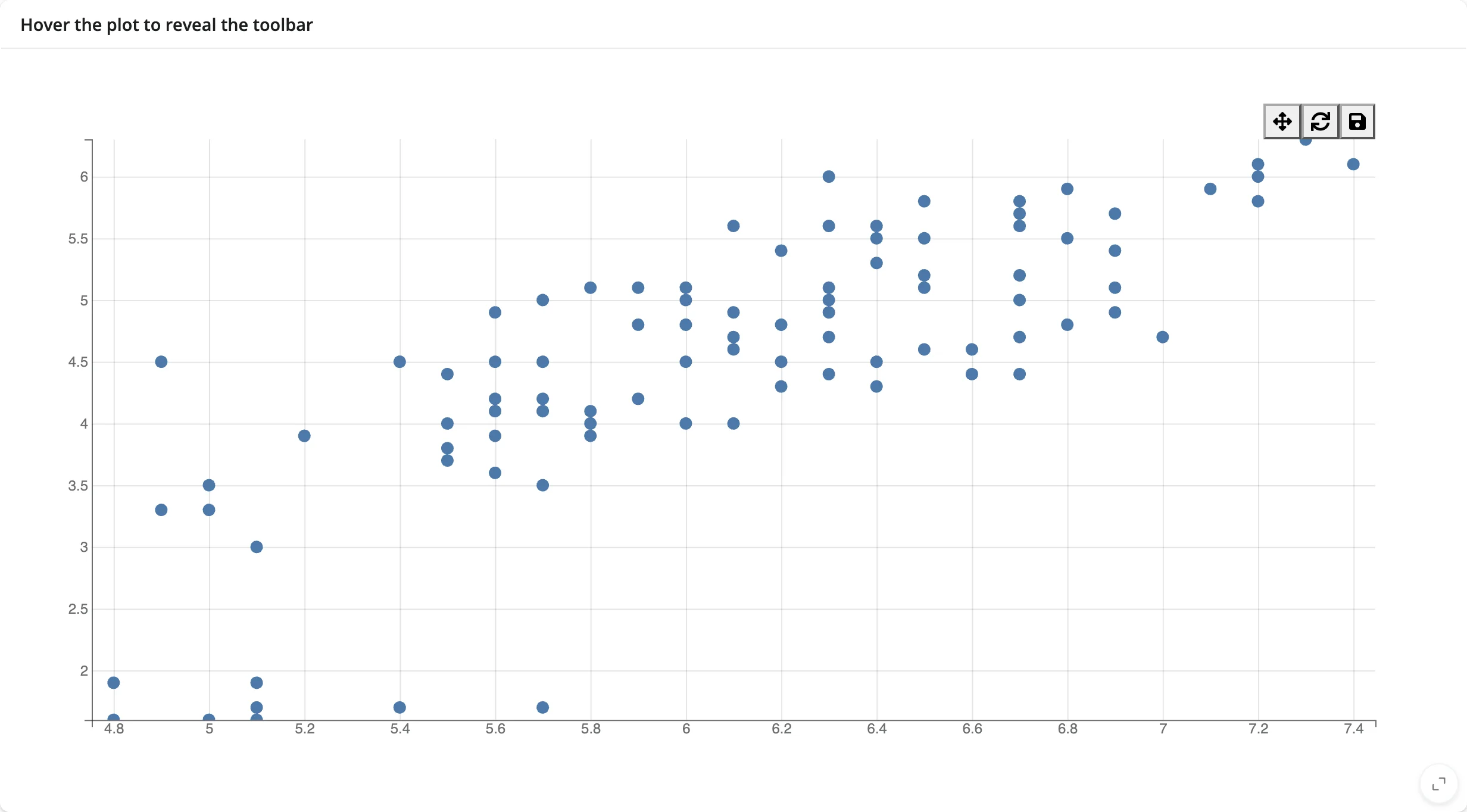
Read the zoomed domain back with reactive_read(scale, ["min", "max"]) – see Beyond the accessors.
Seven selectors, one trait
bqplot ships BrushSelector, BrushIntervalSelector, FastIntervalSelector, IndexSelector, LassoSelector, MultiSelector, and PanZoom – all of them just values of a figure’s interaction trait. Swapping tools is one assignment, no re-render, and selected()/brush() pick up whichever selector is active.
# Seven interaction selectors share the same trait, fig.interaction, so
# swapping tools is one assignment -- no re-render, selected() picks up the
# new selector automatically.
import bqplot
import bqplot.interacts as interacts
import plotly.express as px
from shiny import reactive
from shiny.express import input, render, ui
from shinywidgets import render_bqplot

ui.page_opts(title="Selectors", fillable=True)

iris = px.data.iris()
x_sc, y_sc = bqplot.LinearScale(), bqplot.LinearScale()
scatter = bqplot.Scatter(
    x=iris["sepal_length"],
    y=iris["petal_length"],
    scales={"x": x_sc, "y": y_sc},
    colors=["#4c78a8"],
    selected_style={"fill": "#e45756", "stroke": "black"},
)

ui.input_radio_buttons(
    "tool", "Selector", ["Brush", "Lasso", "Index"], inline=True
)

with ui.layout_columns(col_widths=[8, 4]):
    with ui.card(full_screen=True):

        @render_bqplot
        def plot():
            return bqplot.Figure(
                marks=[scatter],
                axes=[bqplot.Axis(scale=x_sc), bqplot.Axis(scale=y_sc, orientation="vertical")],
                interaction=interacts.BrushSelector(
                    x_scale=x_sc, y_scale=y_sc, marks=[scatter]
                ),
            )

    with ui.card():
        ui.card_header("Selected rows")

        @render.code
        def n_selected():
            sel = plot.selected()[0]
            return "none" if sel is None else f"{len(sel)} point(s)"


@reactive.effect
def _swap_selector():
    tool = input.tool()
    if tool == "Brush":
        new = interacts.BrushSelector(x_scale=x_sc, y_scale=y_sc, marks=[scatter])
    elif tool == "Lasso":
        new = interacts.LassoSelector(x_scale=x_sc, y_scale=y_sc, marks=[scatter])
    else:
        new = interacts.IndexSelector(scale=x_sc, marks=[scatter])
    plot.widget.interaction = new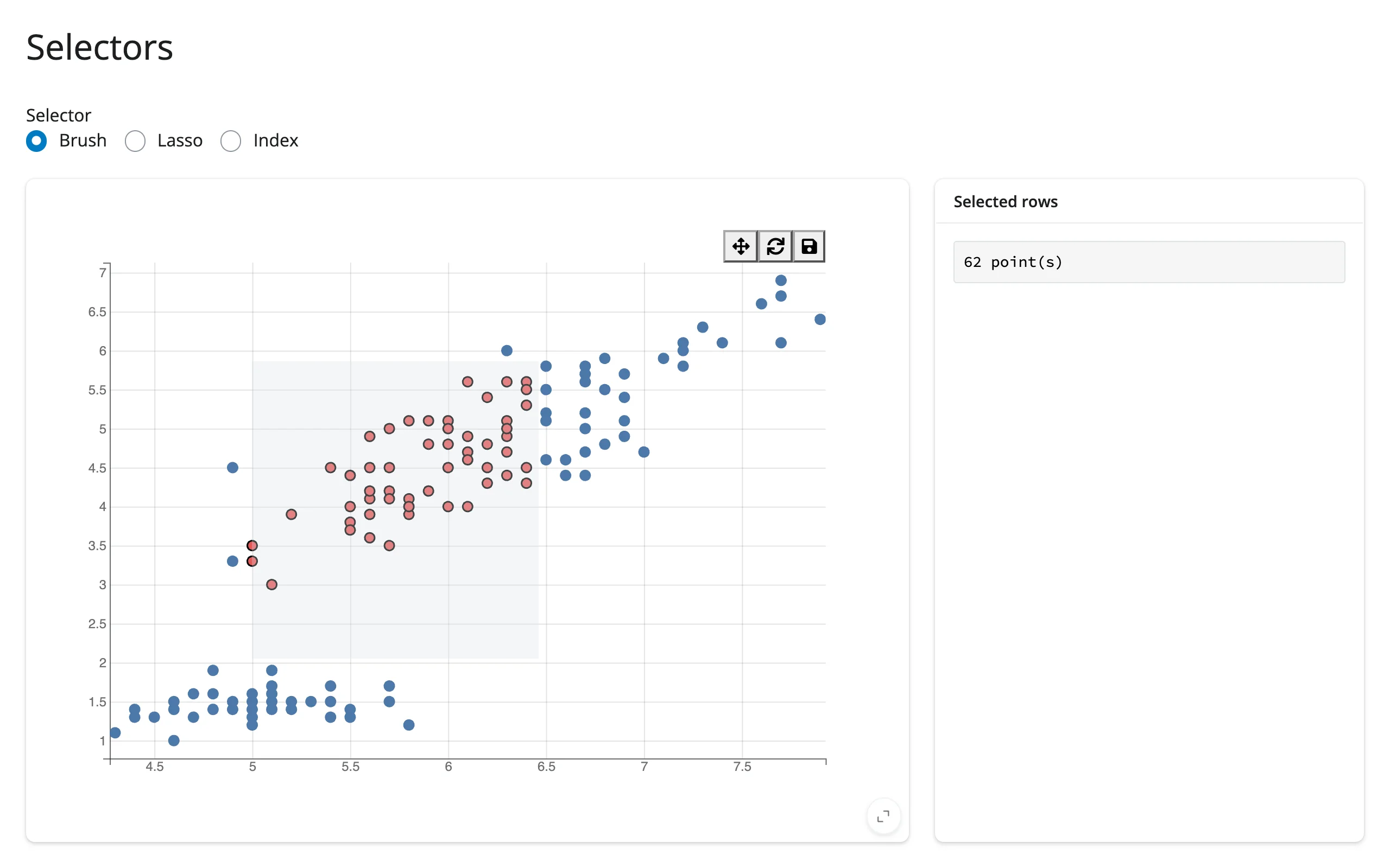
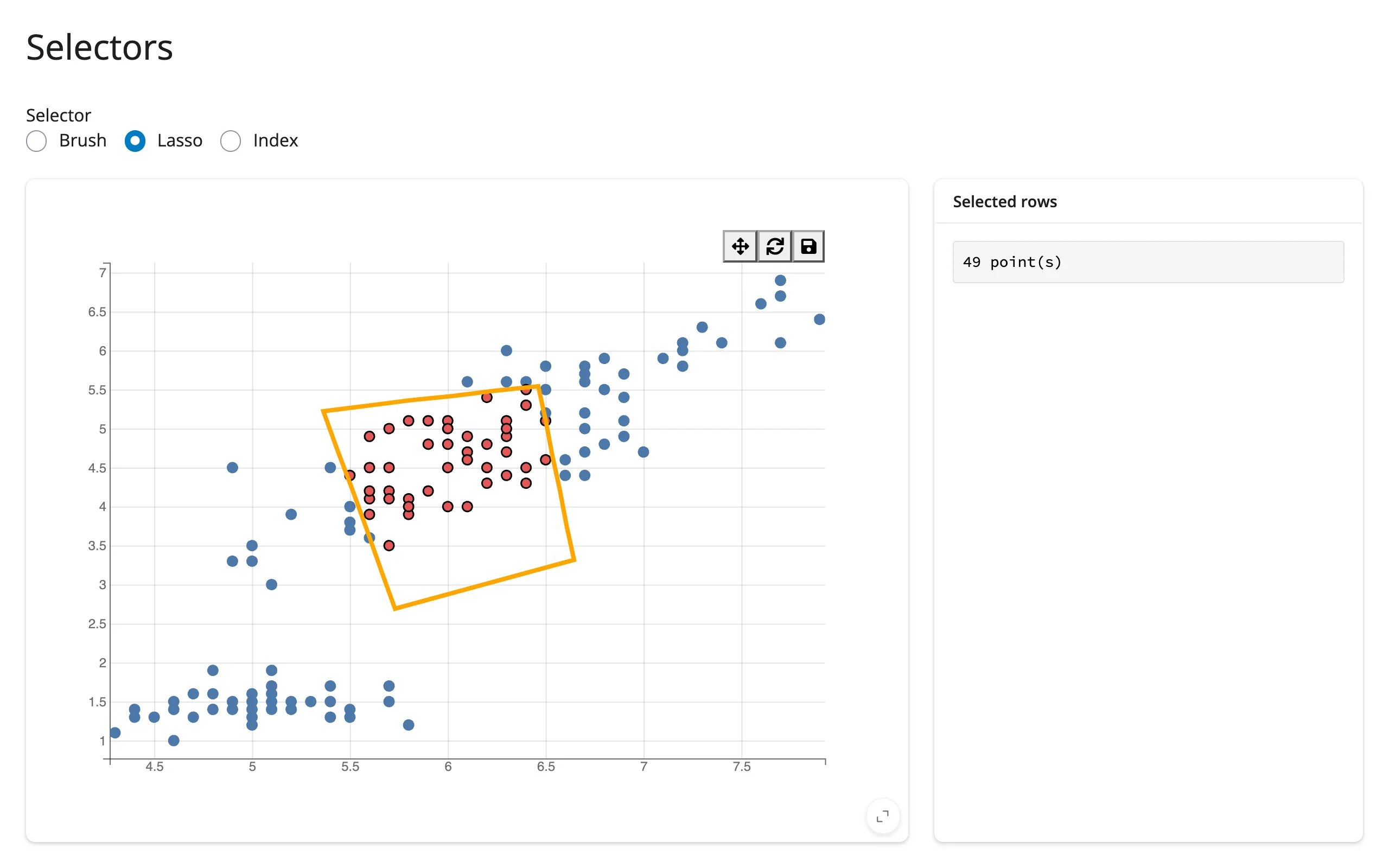
FastIntervalSelector and IndexSelector need one click to activate before they track the mouse – that’s upstream bqplot behavior, not a bug. PanZoom and LassoSelector have no selected region to report, which is why brush() returns None while either is active (see the accessor reference below).
Reacting to user interaction
Accessor reference
| accessor | returns | before any interaction | across re-render | default rate policy |
|---|---|---|---|---|
selected() |
list[numpy.ndarray \| None], one entry per mark in fig.marks |
seeded from each mark’s current selected (None per mark with no selection) |
re-seeded: a new figure’s marks start unselected | debounced, 250 ms |
selected_rows(df, *, mark=None) |
the rows of df (pandas, polars, …; same type out) at one mark’s selected positions; mark is an index into fig.marks or the Mark itself, omittable for single-mark figures |
empty frame (cancels when selected() does) |
derived from selected() |
debounced, 250 ms (follows selected()) |
brush() |
the active selector’s own selected region: a 2x2 array (BrushSelector), a length-2 array (BrushIntervalSelector), a dict of named intervals (MultiSelector), or None |
seeded from the figure’s current interaction (None if nothing is brushed, or interaction isn’t a brush-family selector) |
re-seeded from the new figure’s interaction |
debounced, 250 ms |
Both accessors attach the moment the figure renders – no warm-up read needed – and both re-seed on every re-render, when fig.marks is replaced, or when fig.interaction is swapped (as the toolbar does, or as the selector example above does): a figure’s selection and brush are its own current state, not a record of what the user did, so you never read a stale value left over from a previous figure. There is deliberately no clicked() accessor: a selector’s drag overlay intercepts real clicks on the marks underneath it, so a click accessor would be silently dead whenever a selector is active; mark.on_element_click() remains available for selector-free figures.
selected(): brush, lasso, or click-select
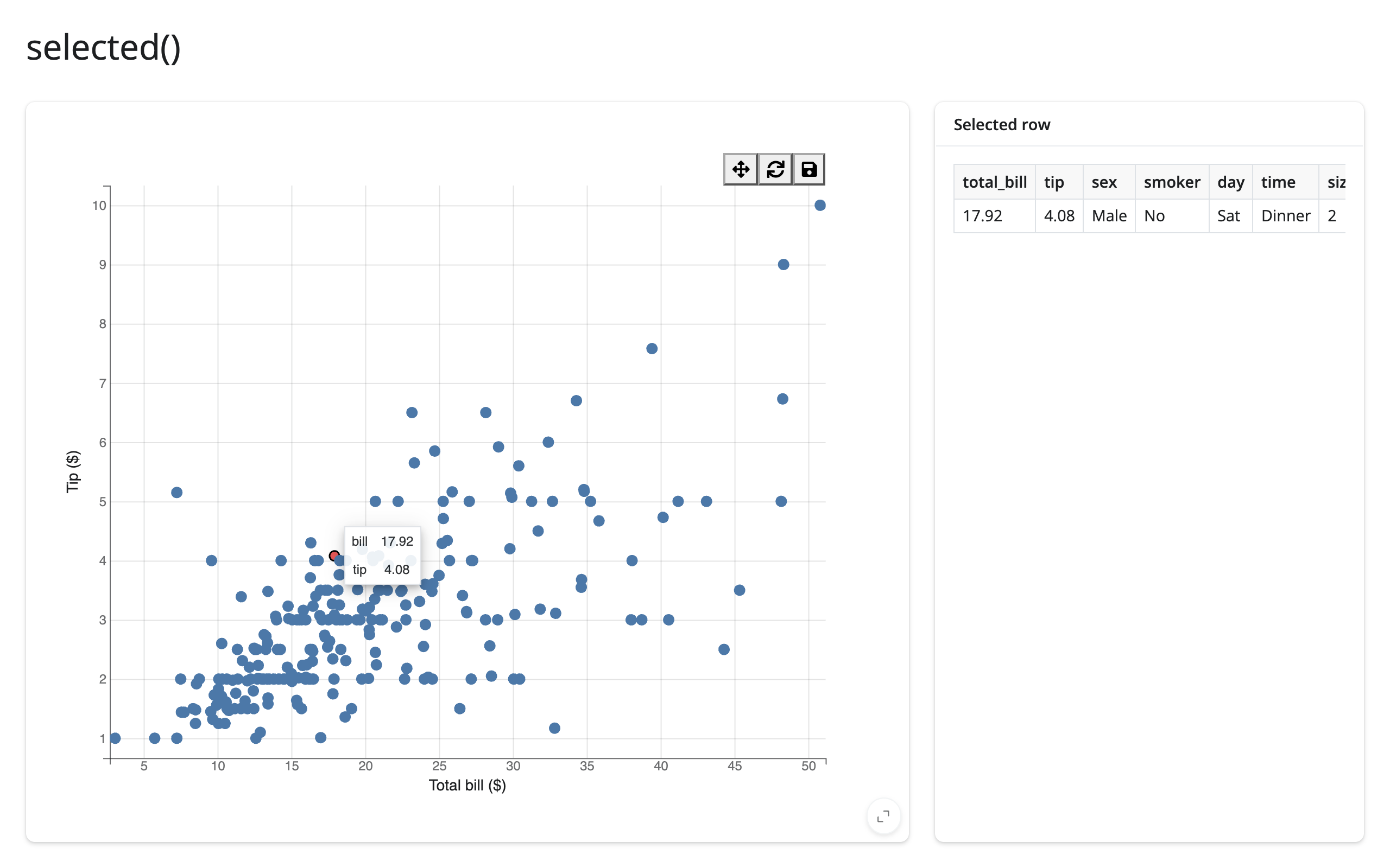
selected() is a list aligned with fig.marks; a single-mark figure reads fig.selected()[0]. It works identically whether the figure’s interaction is a brush, a lasso, or plain click-select (interactions={"click": "select"}, which replaces the mark’s default hover tooltip – add "hover": "tooltip" back if you want both).
# selected() tracks each mark's selected elements. Click-select needs
# interactions={"click": "select"} -- and that replaces the default hover
# tooltip, so add "hover": "tooltip" back if you still want it.
import bqplot
import plotly.express as px
from shiny.express import render, ui
from shinywidgets import render_bqplot

ui.page_opts(title="selected()", fillable=True)

tips = px.data.tips()

with ui.layout_columns(col_widths=[8, 4]):
    with ui.card(full_screen=True):

        @render_bqplot
        def plot():
            x_sc, y_sc = bqplot.LinearScale(), bqplot.LinearScale()
            scatter = bqplot.Scatter(
                x=tips["total_bill"],
                y=tips["tip"],
                scales={"x": x_sc, "y": y_sc},
                colors=["#4c78a8"],
                selected_style={"fill": "#e45756", "stroke": "black"},
                interactions={"click": "select", "hover": "tooltip"},
                tooltip=bqplot.Tooltip(fields=["x", "y"], labels=["bill", "tip"]),
            )
            return bqplot.Figure(
                marks=[scatter],
                axes=[
                    bqplot.Axis(scale=x_sc, label="Total bill ($)"),
                    bqplot.Axis(scale=y_sc, orientation="vertical", label="Tip ($)"),
                ],
            )

    with ui.card():
        ui.card_header("Selected row")

        @render.data_frame
        def detail():
            # empty while nothing is selected; the figure has one mark, so
            # mark= can be omitted
            return plot.selected_rows(tips)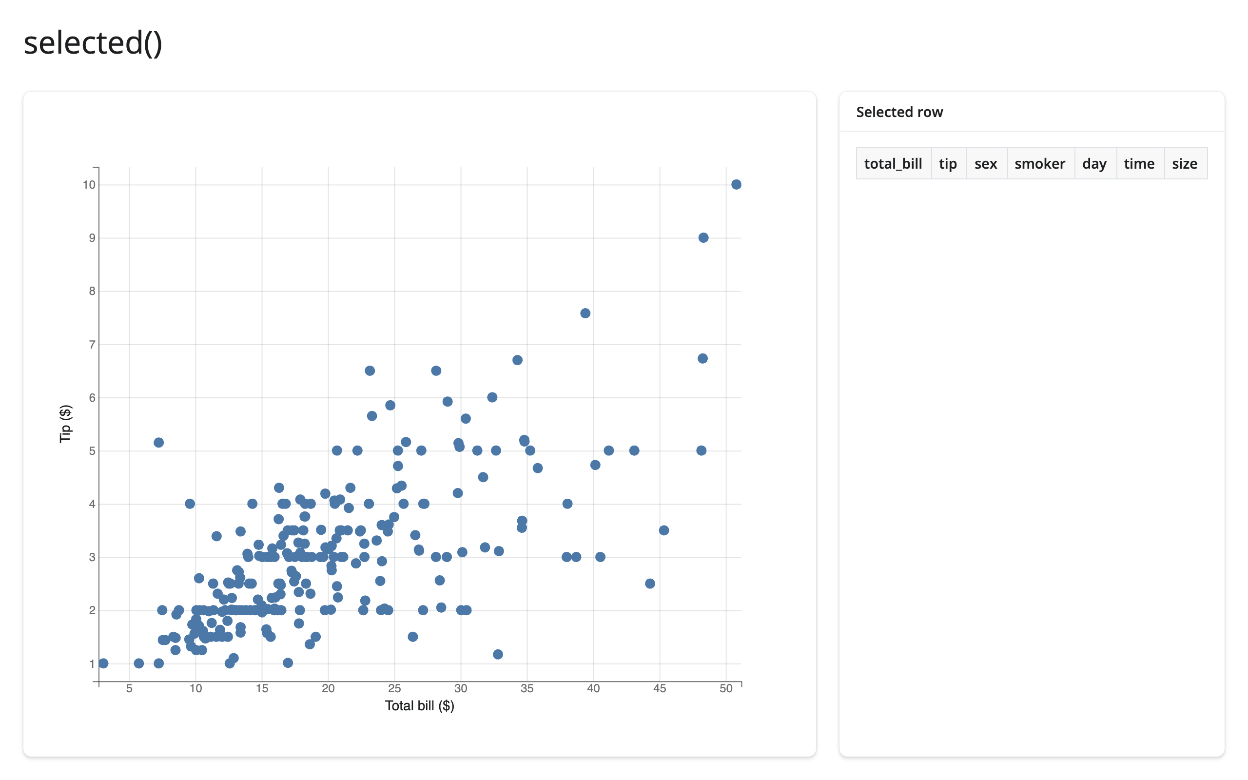
selected_rows(): the selection, as rows of your data frame
When what you want is the selected rows – for a table, a download, or a detail card – selected_rows(df) is the accessor: it maps one mark’s selection back into df and returns those rows, in df’s own type (pandas in, pandas out; polars in, polars out). df is required – a bqplot figure retains no data frame – and it’s an empty frame while the mark has nothing selected, so it can be passed straight to @render.data_frame (the table in the example above).
mark says which mark’s selection maps to df’s rows: its index in fig.marks (mark=1) or the Mark object itself (mark=scatter). Omit it when the figure has exactly one mark; with several marks, omitting it is an error that tells you to pass mark=. The match is positional, like df.iloc[fig.selected()[i]] – after a re-render or in-place data replacement (mark.x = ...) with different rows, a retained position can point at a different row, so carry an ID column and look rows up by it when the data can change.
brush(): the selector’s own region
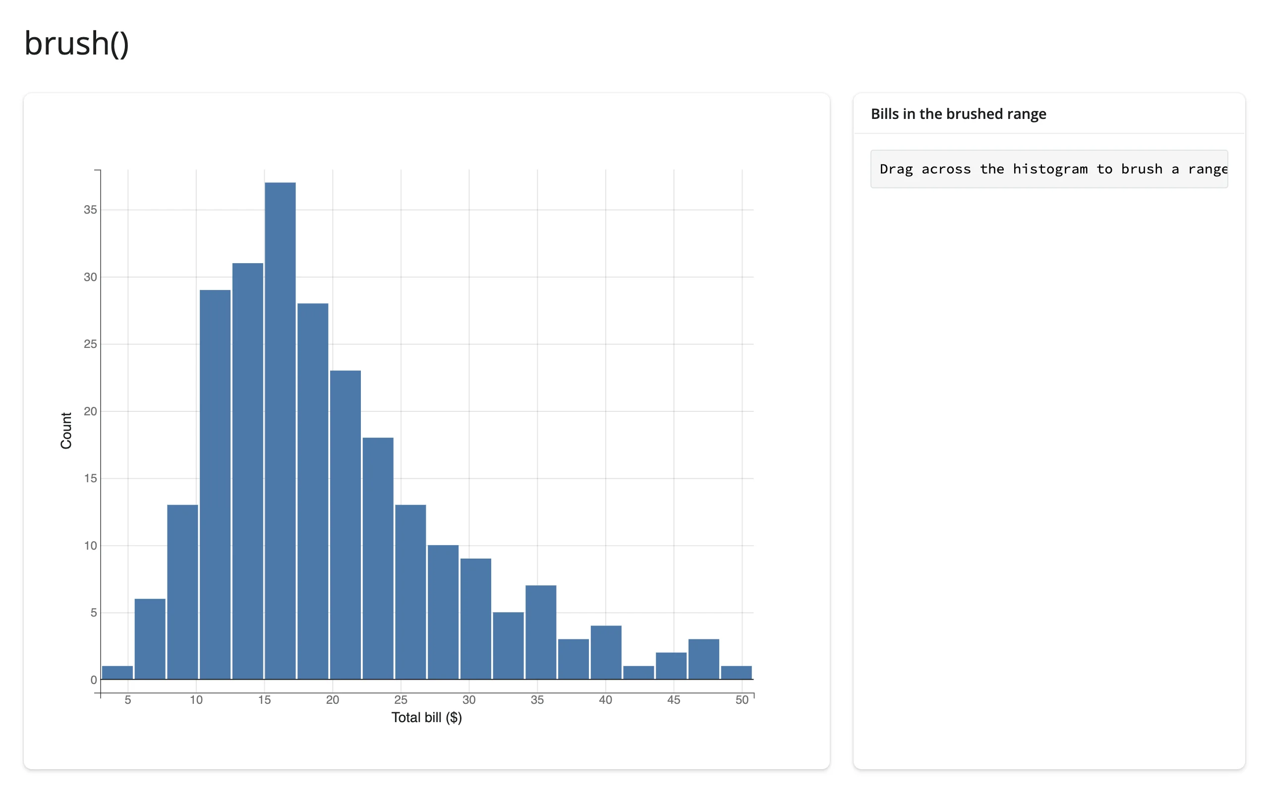
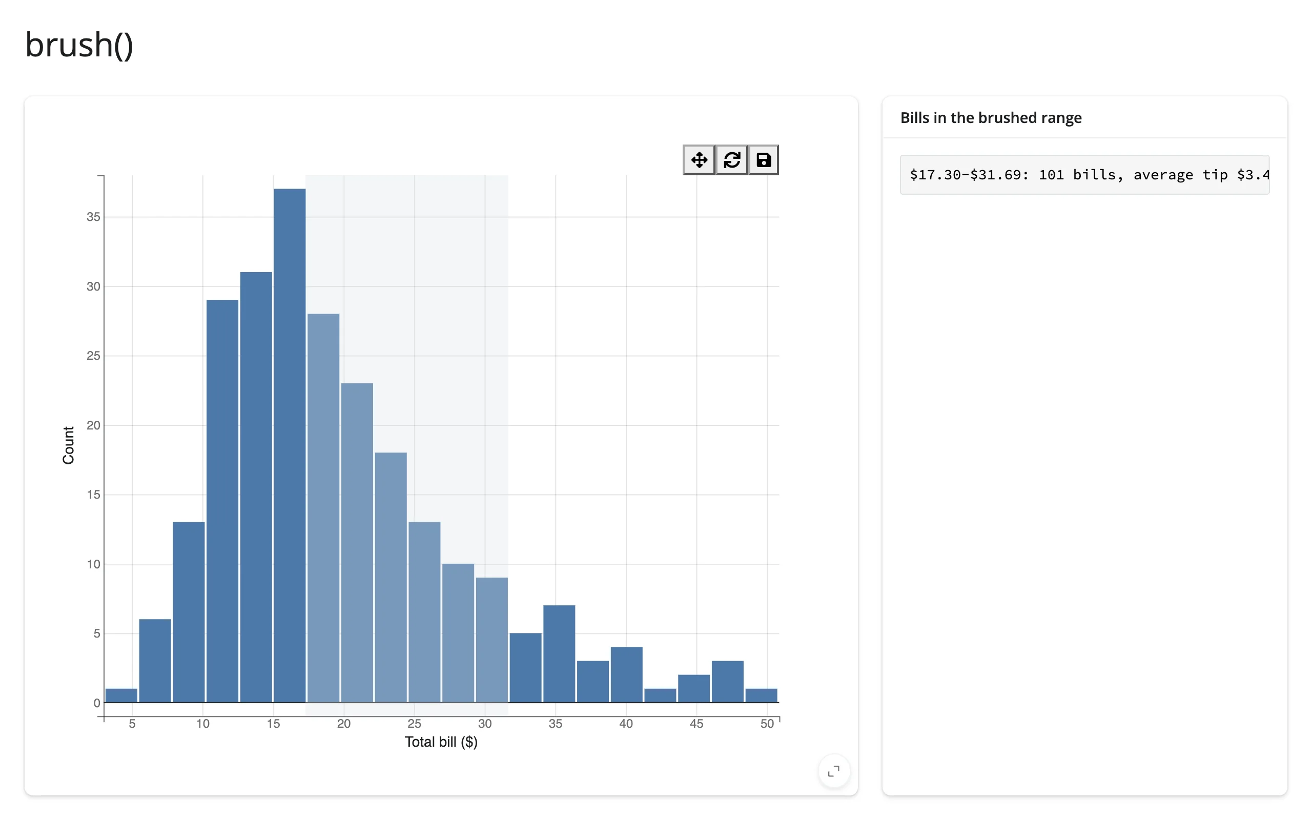
brush() is not row indices – it’s the brush/interval’s own numeric bounds, in data coordinates. Use it when you want the range itself (to filter a different data frame, label an axis, or query a database), rather than which points fall inside it.
# brush() reports the active brush selector's own region, in data
# coordinates -- not row indices. Use it to filter a data frame yourself.
import bqplot
from bqplot.interacts import BrushIntervalSelector
import plotly.express as px
from shiny.express import render, ui
from shinywidgets import render_bqplot

ui.page_opts(title="brush()", fillable=True)

tips = px.data.tips()

with ui.layout_columns(col_widths=[8, 4]):
    with ui.card(full_screen=True):

        @render_bqplot
        def plot():
            x_sc, y_sc = bqplot.LinearScale(), bqplot.LinearScale()
            hist = bqplot.Bins(
                sample=tips["total_bill"],
                scales={"x": x_sc, "y": y_sc},
                colors=["#4c78a8"],
                bins=20,
            )
            return bqplot.Figure(
                marks=[hist],
                axes=[
                    bqplot.Axis(scale=x_sc, label="Total bill ($)"),
                    bqplot.Axis(scale=y_sc, orientation="vertical", label="Count"),
                ],
                interaction=BrushIntervalSelector(scale=x_sc, marks=[hist]),
            )

    with ui.card():
        ui.card_header("Bills in the brushed range")

        @render.code
        def summary():
            region = plot.brush()
            if region is None:
                return "Drag across the histogram to brush a range."
            lo, hi = sorted(region.tolist())
            in_range = tips[tips["total_bill"].between(lo, hi)]
            return (
                f"${lo:.2f}-${hi:.2f}: {len(in_range)} bills, "
                f"average tip ${in_range['tip'].mean():.2f}"
            )
Beyond the accessors: reactive_read
selected() and brush() cover the two traits most apps need, but any trait on the figure, a mark, a scale, or the active interaction is readable with reactive_read(). A mark, a scale, and a selector are all objects nested inside the figure, not the figure widget itself (fig.widget), so fig.read(...) – which only looks at fig.widget’s own traits – can’t reach them; reactive_read() on the specific sub-object is the right tool. Two traits worth knowing:
brushingon brush-family selectors isTrueonly while the mouse button is down. Gate expensive downstream work on it going back toFalserather than recomputing on every intermediate drag position.- A
PanZoom’s scales report the zoomed-in domain as the user pans:reactive_read(scale, "min")and"max"give the currently visible range,Noneuntil the user has zoomed at least once.
# Beyond the accessors: reactive_read() on any trait. "brushing" is True only
# while the mouse button is down, so gate expensive work on it going False.
# A PanZoom's scales report the zoomed-in domain as the user pans.
import bqplot
from bqplot.interacts import BrushIntervalSelector, PanZoom
import numpy as np
from shiny import req
from shiny.express import render, ui
from shinywidgets import reactive_read, render_bqplot

ui.page_opts(title="reactive_read()", fillable=True)

rng = np.random.default_rng(0)
x = np.sort(rng.uniform(0, 100, 500))
y = rng.normal(0, 1, 500).cumsum()

with ui.layout_columns():
    with ui.card():
        ui.card_header('Gate on "brushing" to skip mid-drag work')

        @render_bqplot
        def brushed():
            x_sc, y_sc = bqplot.LinearScale(), bqplot.LinearScale()
            line = bqplot.Lines(x=x, y=y, scales={"x": x_sc, "y": y_sc})
            return bqplot.Figure(
                marks=[line],
                interaction=BrushIntervalSelector(scale=x_sc, marks=[line]),
            )

        @render.code
        def gated_mean():
            brush = brushed.widget.interaction
            selected = reactive_read(brush, "selected")
            req(selected is not None)
            req(not reactive_read(brush, "brushing"))  # wait for mouseup
            lo, hi = sorted(selected.tolist())
            mask = (x >= lo) & (x <= hi)
            return f"mean y in [{lo:.1f}, {hi:.1f}]: {y[mask].mean():.2f}"

    with ui.card():
        ui.card_header("Read the zoomed domain from PanZoom")

        @render_bqplot
        def zoomable():
            x_sc, y_sc = bqplot.LinearScale(), bqplot.LinearScale()
            line = bqplot.Lines(x=x, y=y, scales={"x": x_sc, "y": y_sc})
            return bqplot.Figure(
                marks=[line],
                interaction=PanZoom(scales={"x": [x_sc], "y": [y_sc]}),
            )

        @render.code
        def visible_domain():
            x_sc = zoomable.widget.marks[0].scales["x"]
            lo = reactive_read(x_sc, "min")
            hi = reactive_read(x_sc, "max")
            return f"visible x range: {lo}-{hi}" if lo is not None else "unzoomed"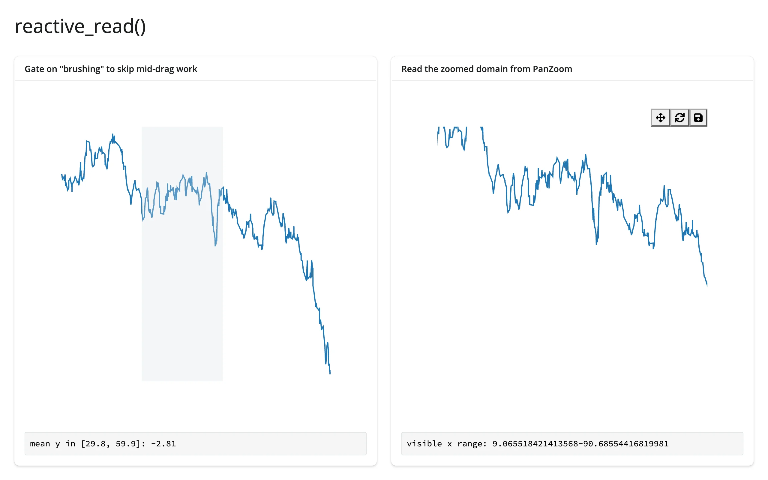
Rate limiting
Both accessors debounce at 250 ms by default, because brush and lasso selectors stream updates throughout the drag, not just at release. Pass rate_policy="throttle" (evenly spaced updates during the gesture) or rate_delay= (seconds; 0 disables rate limiting) to the decorator to change this per output. The same reactive_read() calls are unaffected unless you pass rate_delay too.
# Accessors default to a 250ms debounce (brush selectors stream updates
# mid-drag). rate_policy/rate_delay on the decorator change that per output.
import bqplot
from bqplot.interacts import BrushIntervalSelector
import numpy as np
from shiny.express import render, ui
from shinywidgets import render_bqplot

ui.page_opts(title="Rate limiting", fillable=True)

x = np.linspace(0, 10, 200)
y = np.sin(x)


def make_fig():
    x_sc, y_sc = bqplot.LinearScale(), bqplot.LinearScale()
    line = bqplot.Lines(x=x, y=y, scales={"x": x_sc, "y": y_sc})
    return bqplot.Figure(
        marks=[line], interaction=BrushIntervalSelector(scale=x_sc, marks=[line])
    )


# Plain counters, not reactive.value: a render function may not write to a
# reactive value it also reads, or it retriggers itself in a tight loop
counts = {"debounced": 0, "throttled": 0}

with ui.layout_columns():
    with ui.card():
        ui.card_header("Default: debounce, 250ms")

        @render_bqplot
        def debounced():
            return make_fig()

        @render.code
        def debounced_label():
            debounced.brush()
            counts["debounced"] += 1
            return f"brush() re-fired {counts['debounced']} times"

    with ui.card():
        ui.card_header('rate_policy="throttle", rate_delay=0.05')

        @render_bqplot(rate_policy="throttle", rate_delay=0.05)
        def throttled():
            return make_fig()

        @render.code
        def throttled_label():
            throttled.brush()
            counts["throttled"] += 1
            return f"brush() re-fired {counts['throttled']} times"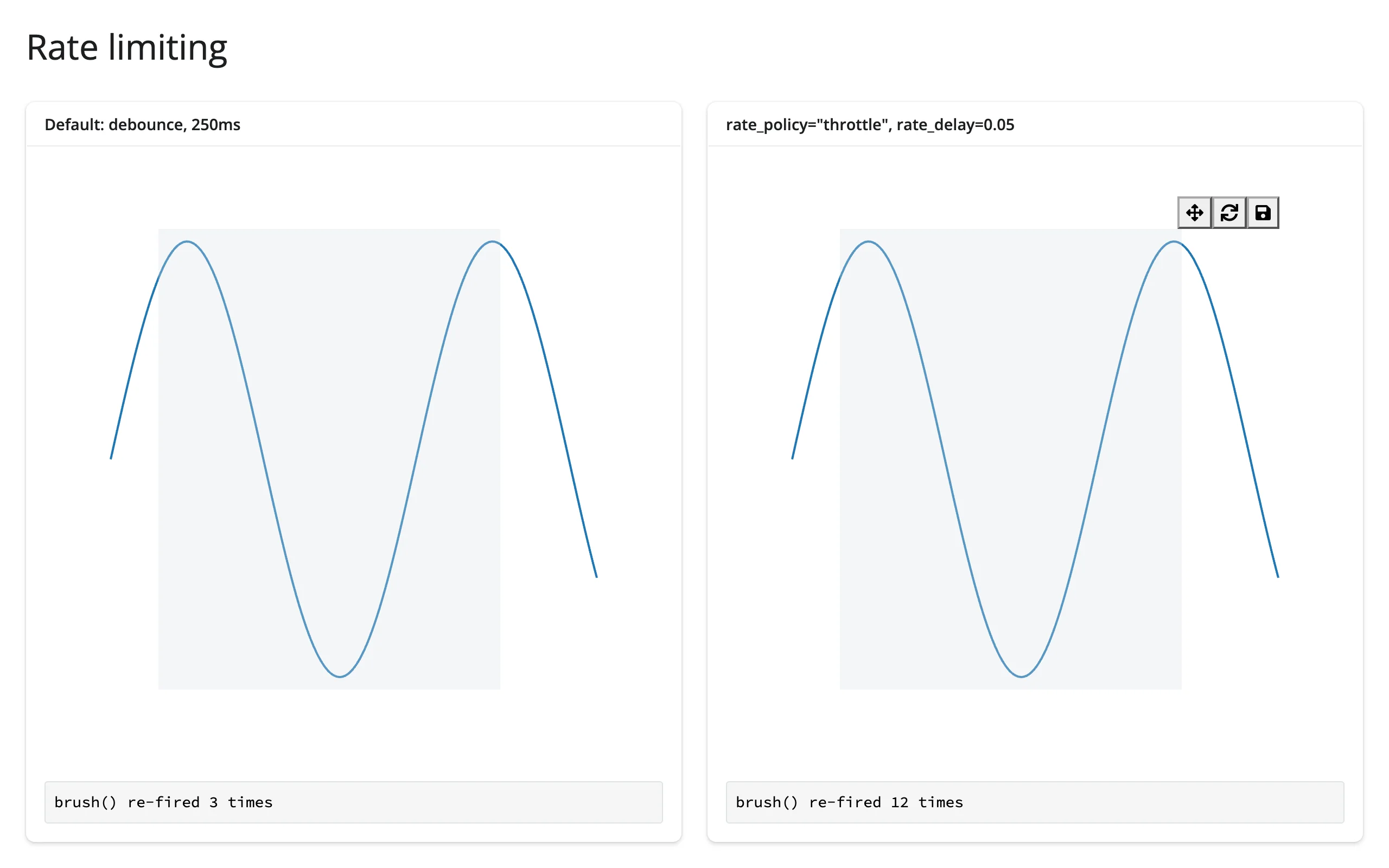
Driving the same drag gesture at both panels: the debounced panel settled after 4 updates, the 50 ms throttle fired 14 times during the same drag.
Reading an accessor on demand
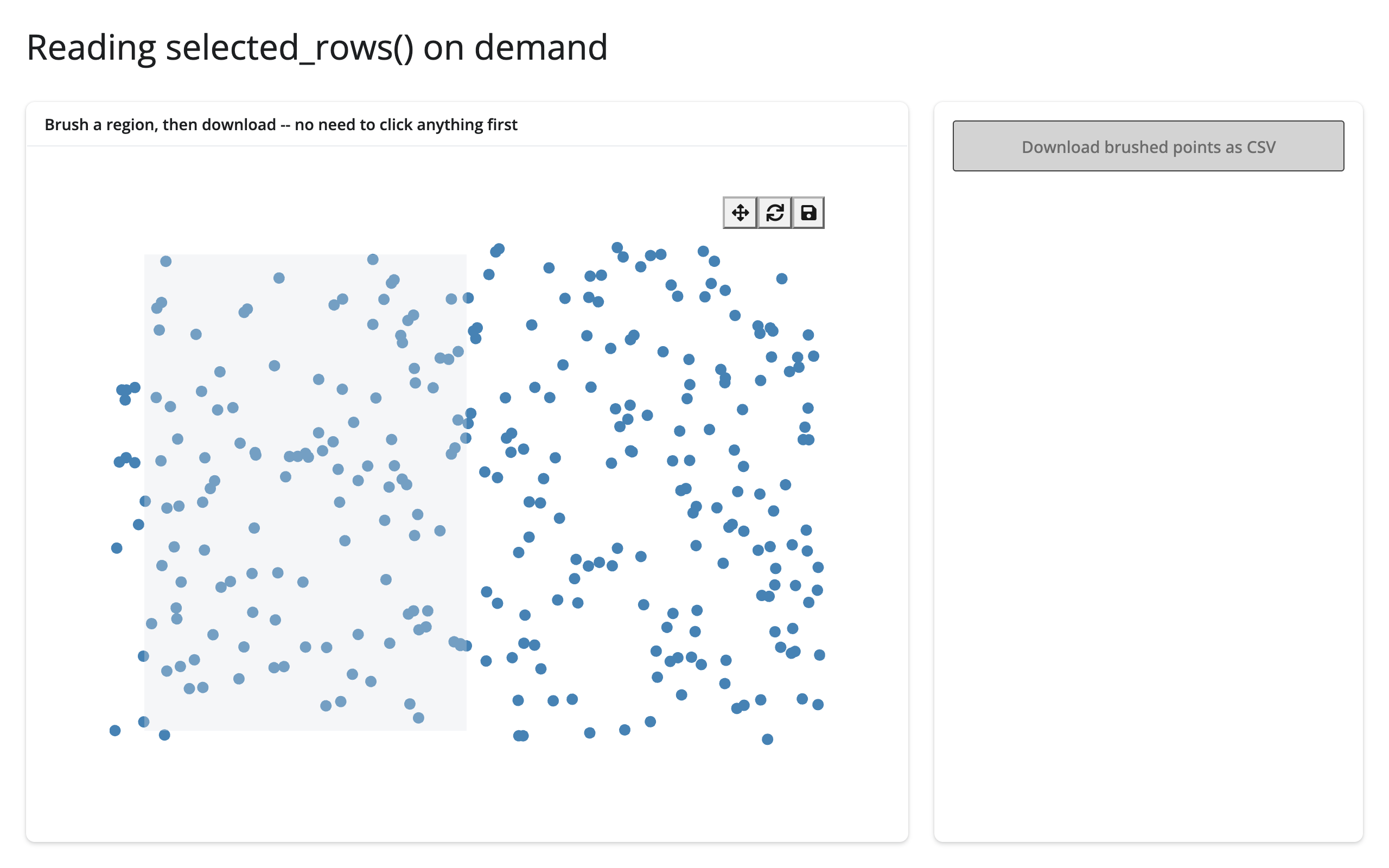
selected_rows() is seeded the moment the figure renders (an empty frame while nothing is selected), so it’s safe to read somewhere that only runs occasionally – a download handler, say – with no prior read needed first:
import bqplot
import numpy as np
import pandas as pd
from bqplot.interacts import BrushSelector
from shiny.express import render, ui
from shinywidgets import render_bqplot

ui.page_opts(title="Reading selected_rows() on demand", fillable=True)

rng = np.random.default_rng(0)
points = pd.DataFrame(
    {"x": rng.uniform(0, 10, 300), "y": rng.uniform(0, 10, 300)}
)
x, y = points["x"], points["y"]

with ui.layout_columns(col_widths=[8, 4]):
    with ui.card(full_screen=True):
        ui.card_header("Brush a region, then download -- no need to click anything first")

        @render_bqplot
        def plot():
            x_sc, y_sc = bqplot.LinearScale(), bqplot.LinearScale()
            scatter = bqplot.Scatter(x=x, y=y, scales={"x": x_sc, "y": y_sc})
            return bqplot.Figure(
                marks=[scatter],
                interaction=BrushSelector(x_scale=x_sc, y_scale=y_sc, marks=[scatter]),
            )

    with ui.card():

        @render.download_button(
            filename="brushed.csv", label="Download brushed points as CSV"
        )
        def download():
            # selected_rows() is live from the moment the figure renders, so
            # this reads whatever's currently brushed, even on its first run.
            yield plot.selected_rows(points).to_csv(index=False)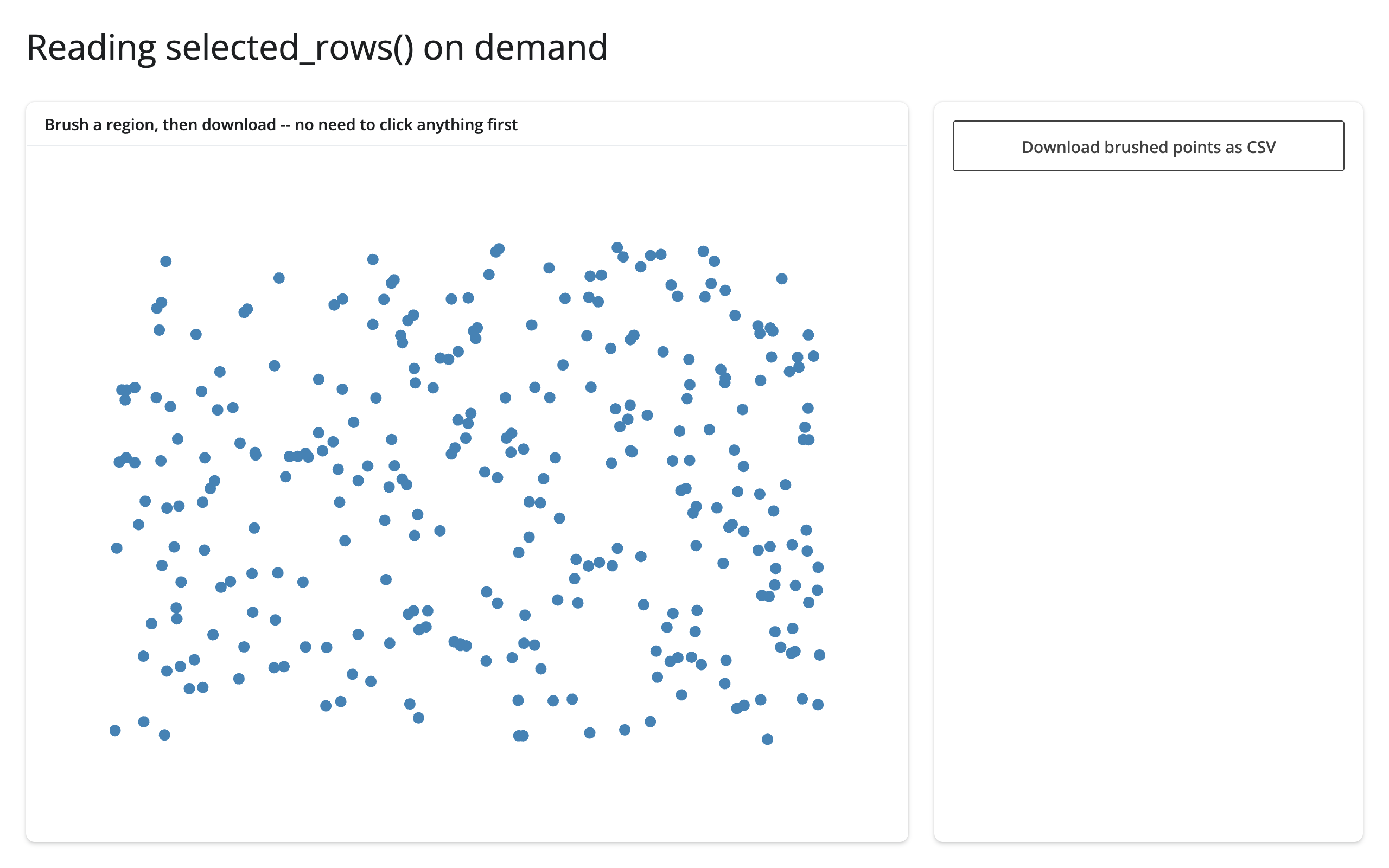
Updating the widget from Python
Two ways to change what a render_bqplot output shows: return a new Figure from the render function (a re-render), or mutate the existing Figure’s traits from an effect or another output (an in-place update). Re-rendering is simpler but throws away everything the user did to the old figure – any PanZoom zoom/pan state, any selection – because a fresh Figure means fresh scales and fresh marks. In-place updates keep the user’s view exactly where it was and, with animation_duration set, animate the change instead of snapping to it.
# Re-rendering rebuilds the figure (and its scales), so any PanZoom state is
# lost. Mutating the existing mark's data preserves zoom/pan and animates.
# reactive.isolate() reads .widget without tying this effect to the render.
import bqplot
import numpy as np
from shiny import reactive
from shiny.express import input, ui
from shinywidgets import render_bqplot

ui.page_opts(title="In-place vs re-render", fillable=True)
ui.input_slider("phase", "Phase shift", 0, 10, 0, step=0.5)

x = np.linspace(0, 10, 200)


def panzoom_fig(y: np.ndarray) -> bqplot.Figure:
    x_sc, y_sc = bqplot.LinearScale(), bqplot.LinearScale()
    line = bqplot.Lines(x=x, y=y, scales={"x": x_sc, "y": y_sc})
    return bqplot.Figure(
        marks=[line], interaction=bqplot.interacts.PanZoom(scales={"x": [x_sc], "y": [y_sc]})
    )


with ui.layout_columns():
    with ui.card(full_screen=True):
        ui.card_header("Re-render: zoom resets on every change")

        @render_bqplot
        def rerendered():
            return panzoom_fig(np.sin(x + input.phase()))

    with ui.card(full_screen=True):
        ui.card_header("In-place: zoom survives, the line animates")

        @render_bqplot
        def inplace():
            # Doesn't depend on input.phase(): built once, edited afterward
            fig = panzoom_fig(np.sin(x))
            fig.animation_duration = 400
            return fig


@reactive.effect
def _update_inplace():
    phase = input.phase()
    with reactive.isolate():
        fig = inplace.widget
    fig.marks[0].y = np.sin(x + phase)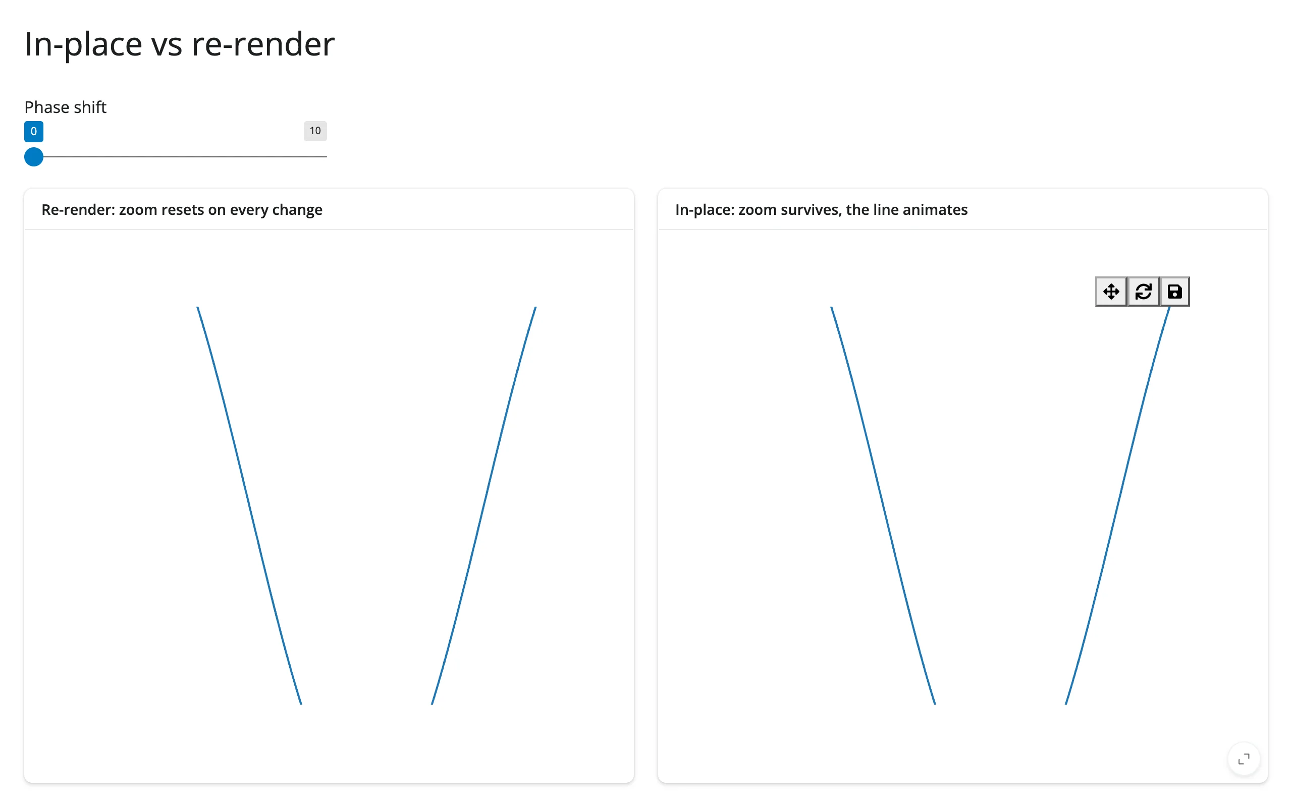
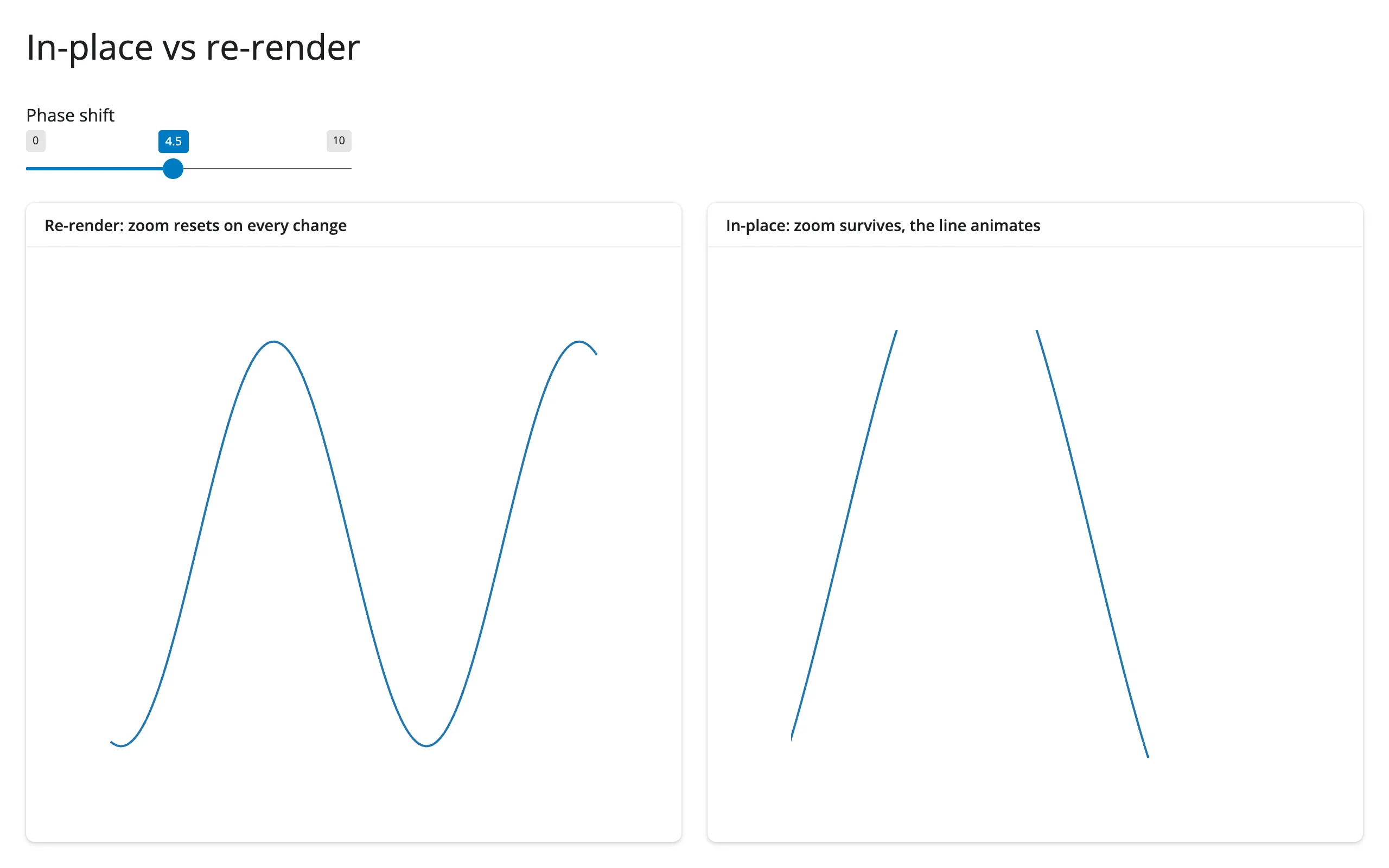
Both panels were zoomed in identically before the phase slider moved. After the change, the re-render panel (left) has snapped back to its full, unzoomed domain; the in-place panel (right) kept the same zoomed-in view and animated the line to its new phase. reactive.isolate() around .widget keeps this effect’s only reactive dependency on input.phase() – reading .widget directly would also make the effect depend on inplace’s own render, which it never needs to.
The gapminder example above uses the same pattern at a larger scale: the figure is built once, with animation_duration set, and a reactive.effect reacting to input.year() is the only thing that ever touches points.x/y/color/size again.
Coordinating multiple views
Brush select → filtered table
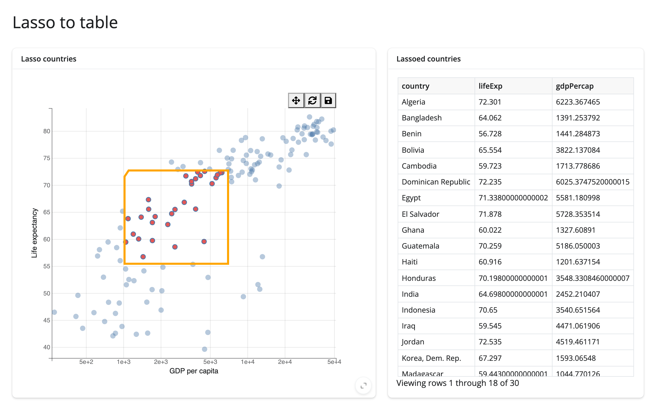
The most direct pattern: read selected_rows(df) and hand the selected rows to render.data_frame. No effects needed, since render.data_frame already re-runs whenever the accessor’s value changes.
# Pattern: lasso select -> filtered table. selected_rows() maps the lasso
# back to rows of the data frame, no manual event wiring.
import bqplot
import bqplot.interacts as interacts
import plotly.express as px
from shiny.express import render, ui
from shinywidgets import render_bqplot

ui.page_opts(title="Lasso to table", fillable=True)

gap2007 = px.data.gapminder().query("year == 2007").reset_index(drop=True)

with ui.layout_columns(col_widths=[7, 5]):
    with ui.card(full_screen=True):
        ui.card_header("Lasso countries")

        @render_bqplot
        def plot():
            x_sc = bqplot.LogScale()
            y_sc = bqplot.LinearScale()
            scatter = bqplot.Scatter(
                x=gap2007["gdpPercap"],
                y=gap2007["lifeExp"],
                scales={"x": x_sc, "y": y_sc},
                colors=["#4c78a8"],
                selected_style={"fill": "#e45756"},
                unselected_style={"opacity": 0.4},
            )
            return bqplot.Figure(
                marks=[scatter],
                axes=[
                    bqplot.Axis(scale=x_sc, label="GDP per capita"),
                    bqplot.Axis(scale=y_sc, orientation="vertical", label="Life expectancy"),
                ],
                interaction=interacts.LassoSelector(
                    x_scale=x_sc, y_scale=y_sc, marks=[scatter]
                ),
            )

    with ui.card():
        ui.card_header("Lassoed countries")

        @render.data_frame
        def table():
            # empty while nothing is lassoed, so it can be passed straight
            # to render.data_frame
            rows = plot.selected_rows(gap2007)
            return render.DataGrid(rows[["country", "lifeExp", "gdpPercap"]])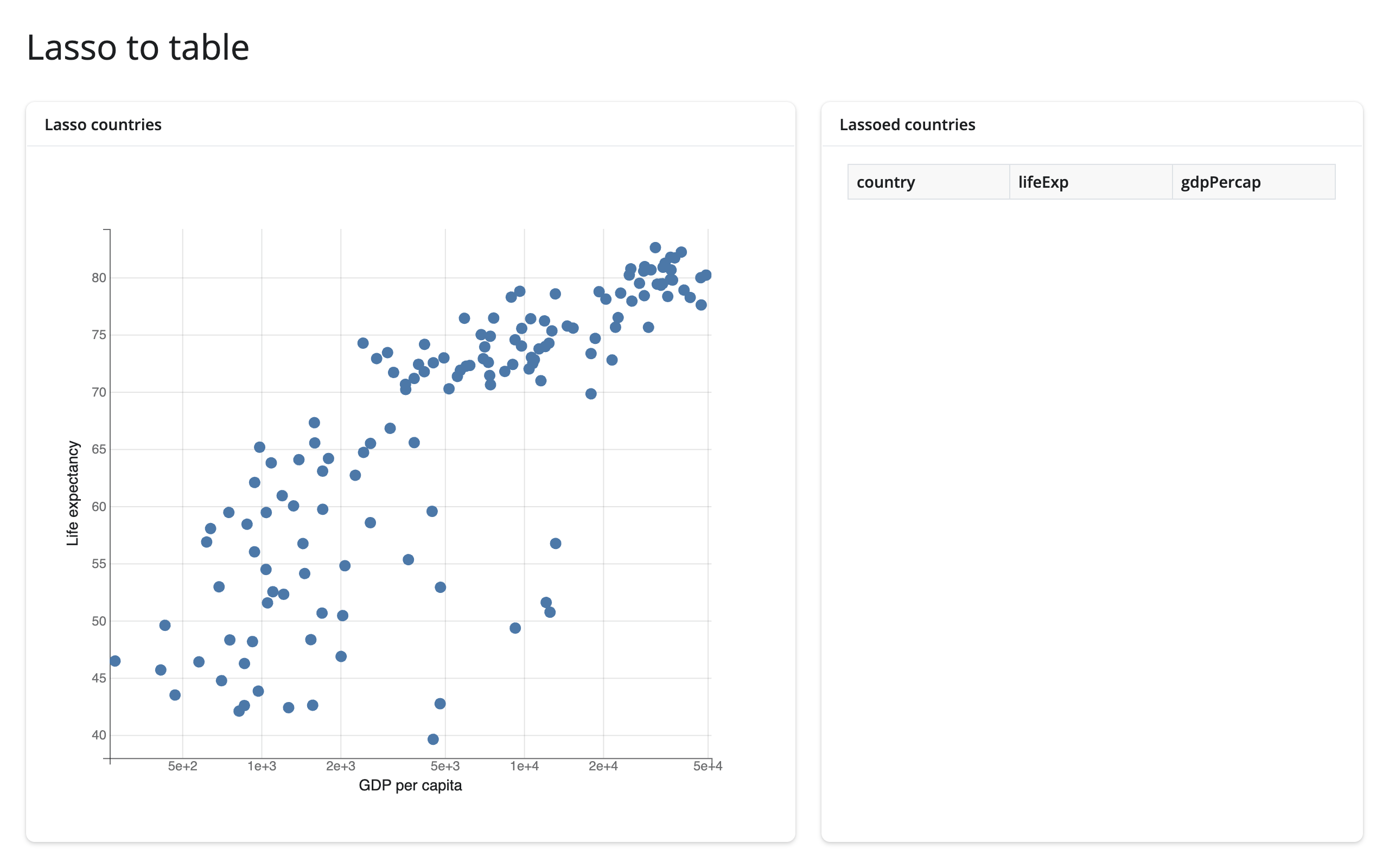
Click → detail card
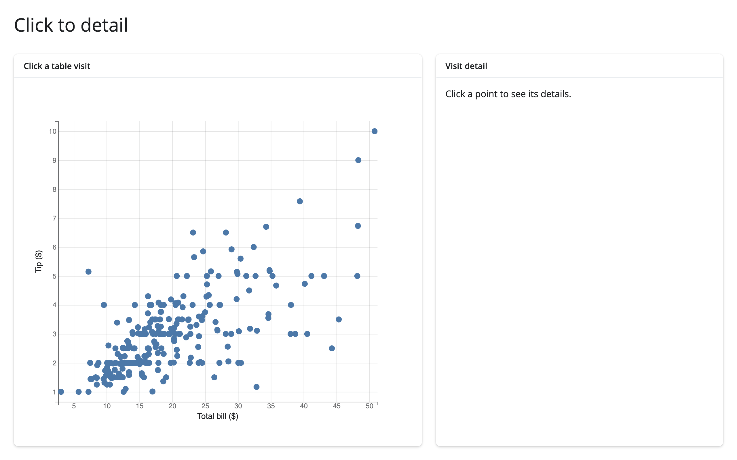
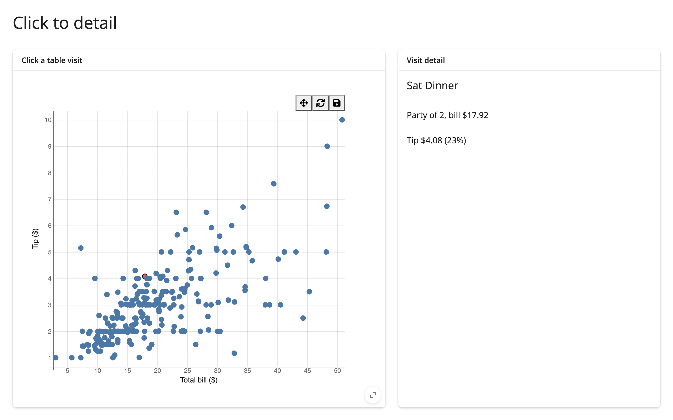
A click-selection is one row of selected_rows(); read it as a scalar row for a detail view.
# Pattern: click a point -> detail card. A single-click selection is one row
# of selected_rows(), so the same accessor drives a 1-row detail view.
import bqplot
import plotly.express as px
from shiny.express import render, ui
from shinywidgets import render_bqplot

ui.page_opts(title="Click to detail", fillable=True)

tips = px.data.tips()

with ui.layout_columns(col_widths=[7, 5]):
    with ui.card(full_screen=True):
        ui.card_header("Click a table visit")

        @render_bqplot
        def plot():
            x_sc, y_sc = bqplot.LinearScale(), bqplot.LinearScale()
            scatter = bqplot.Scatter(
                x=tips["total_bill"],
                y=tips["tip"],
                scales={"x": x_sc, "y": y_sc},
                colors=["#4c78a8"],
                selected_style={"fill": "#e45756", "stroke": "black"},
                interactions={"click": "select", "hover": "tooltip"},
            )
            return bqplot.Figure(
                marks=[scatter],
                axes=[
                    bqplot.Axis(scale=x_sc, label="Total bill ($)"),
                    bqplot.Axis(scale=y_sc, orientation="vertical", label="Tip ($)"),
                ],
            )

    with ui.card():
        ui.card_header("Visit detail")

        @render.ui
        def detail():
            rows = plot.selected_rows(tips)
            if len(rows) == 0:
                return ui.p("Click a point to see its details.")
            row = rows.iloc[0]  # a click selects a single visit
            pct = 100 * row["tip"] / row["total_bill"]
            return ui.TagList(
                ui.h5(f"{row['day']} {row['time']}"),
                ui.p(f"Party of {row['size']}, bill ${row['total_bill']:.2f}"),
                ui.p(f"Tip ${row['tip']:.2f} ({pct:.0f}%)"),
            )
Widget state → another widget updated in place
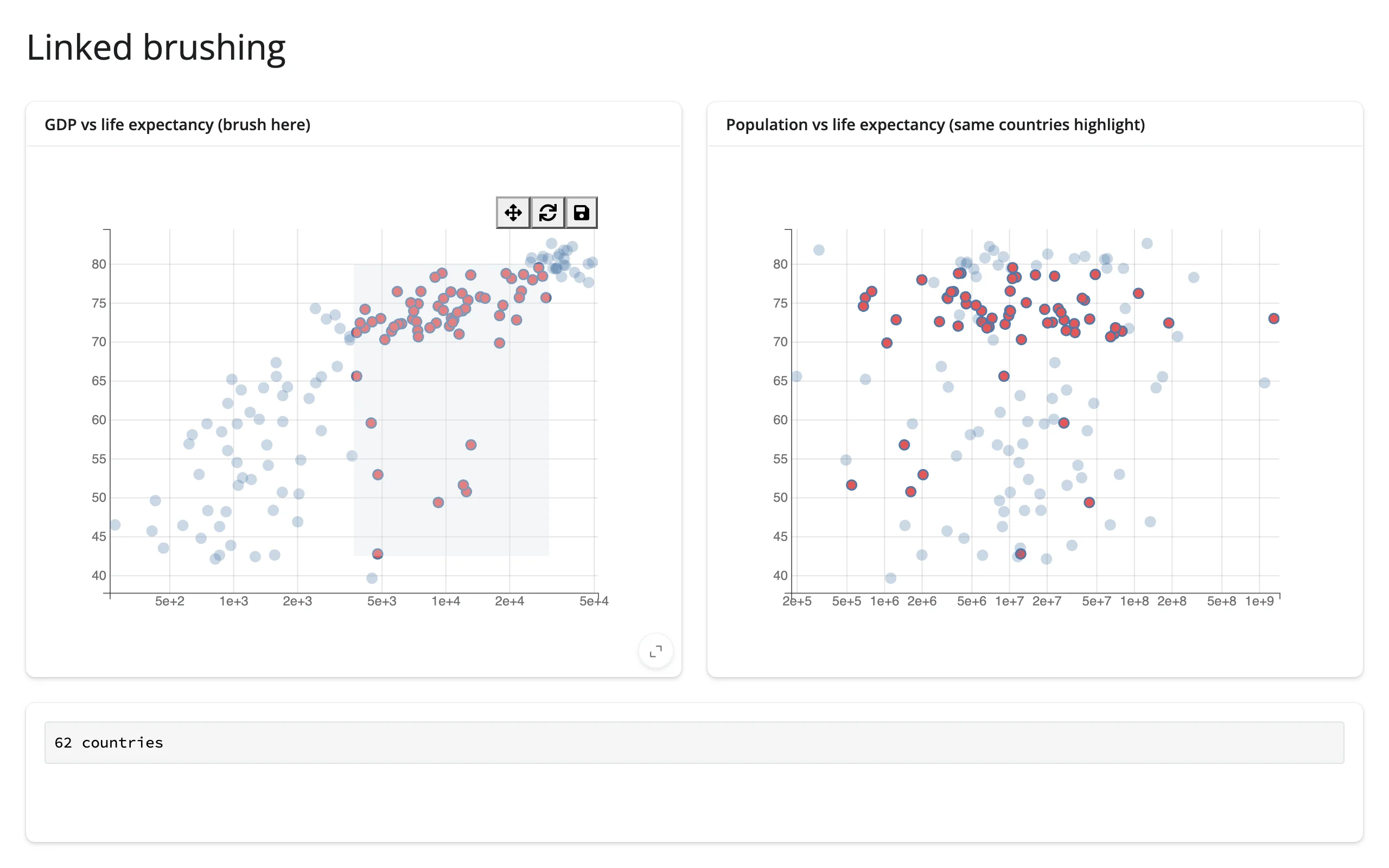
bqplot’s own selectors can only highlight marks on the figure they’re attached to (see Gotchas). To link a second, separately rendered figure, go through Python: read selected() on the first figure, and set .selected on the second figure’s mark from an effect. Nothing re-renders on either side.
# Pattern: widget state -> another widget updated in place. bqplot's own
# selectors can only highlight marks on the figure they're attached to, so
# linking a *second* figure goes through Python: read selected() here, set
# .selected on the other figure's mark in an effect. No re-render either side.
import bqplot
import bqplot.interacts as interacts
import plotly.express as px
from shiny import reactive
from shiny.express import render, ui
from shinywidgets import render_bqplot

ui.page_opts(title="Linked brushing", fillable=True)

gap2007 = px.data.gapminder().query("year == 2007").reset_index(drop=True)
gdp_sc, life_sc, pop_sc = bqplot.LogScale(), bqplot.LinearScale(), bqplot.LogScale()

with ui.layout_columns():
    with ui.card(full_screen=True):
        ui.card_header("GDP vs life expectancy (brush here)")

        @render_bqplot
        def left():
            wealth = bqplot.Scatter(
                x=gap2007["gdpPercap"],
                y=gap2007["lifeExp"],
                scales={"x": gdp_sc, "y": life_sc},
                colors=["#4c78a8"],
                selected_style={"fill": "#e45756"},
                unselected_style={"opacity": 0.3},
            )
            return bqplot.Figure(
                marks=[wealth],
                axes=[bqplot.Axis(scale=gdp_sc), bqplot.Axis(scale=life_sc, orientation="vertical")],
                interaction=interacts.BrushSelector(x_scale=gdp_sc, y_scale=life_sc, marks=[wealth]),
            )

    with ui.card(full_screen=True):
        ui.card_header("Population vs life expectancy (same countries highlight)")

        @render_bqplot
        def right():
            by_pop = bqplot.Scatter(
                x=gap2007["pop"],
                y=gap2007["lifeExp"],
                scales={"x": pop_sc, "y": life_sc},
                colors=["#4c78a8"],
                selected_style={"fill": "#e45756"},
                unselected_style={"opacity": 0.3},
            )
            return bqplot.Figure(
                marks=[by_pop],
                axes=[bqplot.Axis(scale=pop_sc), bqplot.Axis(scale=life_sc, orientation="vertical")],
            )


with ui.card():

    @render.code
    def count():
        sel = left.selected()[0]
        return "no countries brushed" if sel is None else f"{len(sel)} countries"


@reactive.effect
def _highlight_right():
    sel = left.selected()[0]
    with reactive.isolate():
        by_pop = right.widget.marks[0]
    by_pop.selected = sel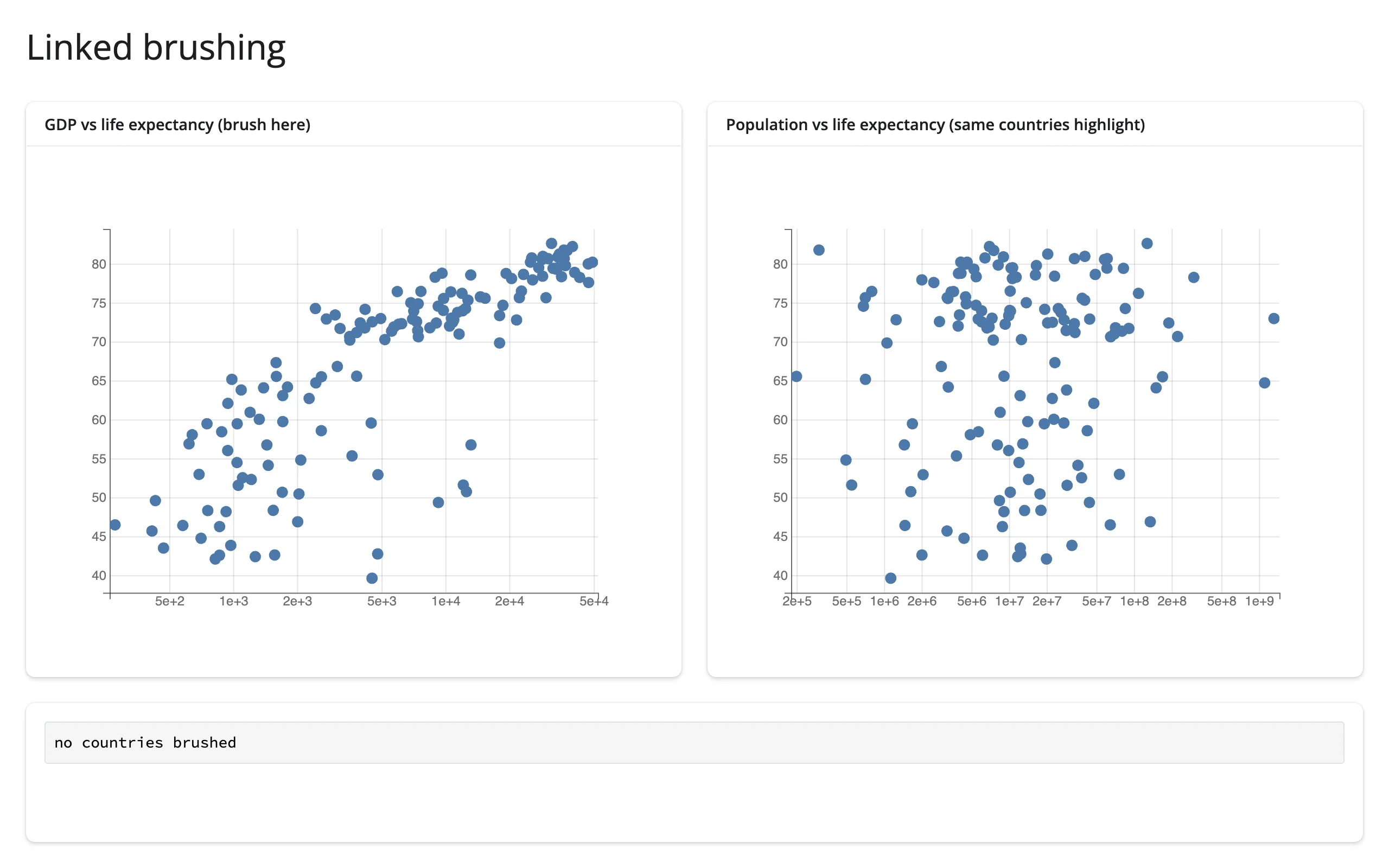
Large data
bqplot has no large-data mode: marks are individual SVG/Canvas elements with no WebGL backend and no server-side rasterization, so every mark the browser draws (and every selector hit-tests) is drawn directly. Upstream bqplot documents no specific row/mark ceiling, and we didn’t measure one this pass. For data that needs to scale into the millions, pair bqplot’s brush/selector interactions with a widget built for scale and drive it from the Python round-trip pattern in Coordinating multiple views above instead of plotting the raw data in bqplot itself – see holoviews+datashader for a density raster or jscatter for a GPU scatter. See Large data & performance for how those compare.
Layout and sizing
A render_bqplot output fills its card by default, the same as every other shinywidgets renderer. render_bqplot(height=...) sets an exact pixel height on the output; Figure(layout={"height": ...}) sets it one level down, on the figure itself, which also opts that figure out of filling its container.
# By default a figure fills its card. render_bqplot(height=...) sets an
# exact pixel height instead; Figure(layout={"height": ...}) does the same
# thing one level down, and also opts the output out of filling.
import bqplot
from shiny.express import ui
from shinywidgets import render_bqplot

ui.page_opts(title="Layout and sizing", fillable=True)


def line_fig(title: str, **kwargs: object) -> bqplot.Figure:
    x_sc, y_sc = bqplot.LinearScale(), bqplot.LinearScale()
    line = bqplot.Lines(x=[1, 2, 3], y=[1, 3, 2], scales={"x": x_sc, "y": y_sc})
    return bqplot.Figure(
        marks=[line],
        axes=[bqplot.Axis(scale=x_sc), bqplot.Axis(scale=y_sc, orientation="vertical")],
        title=title,
        **kwargs,
    )


with ui.layout_columns():
    with ui.card(full_screen=True):
        ui.card_header("Fills the card")

        @render_bqplot
        def fills():
            return line_fig("fill")

    with ui.card():
        ui.card_header("render_bqplot(height=...)")

        @render_bqplot(height="220px")
        def fixed():
            return line_fig("220px")

    with ui.card():
        ui.card_header("Figure(layout={'height': ...})")

        @render_bqplot
        def own_height():
            return line_fig("300px, own layout", layout={"height": "300px"})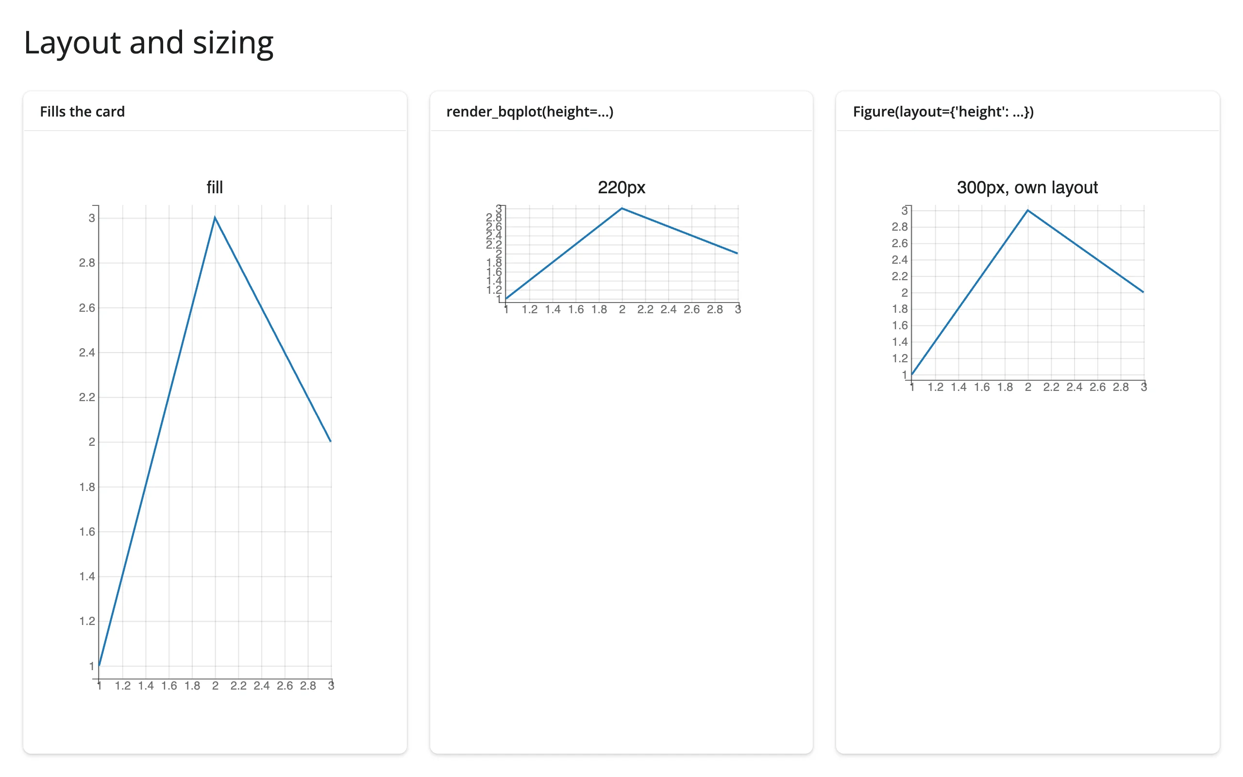
bqplot’s default margins (60px on every side) and fixed axis tick counts don’t adapt to a small card – in a narrow sidebar, pass fig_margin=dict(top=20, bottom=50, left=55, right=15) and reduce Axis(num_ticks=...). Pie and Radar similarly use pixel-based sizing (radius=, and Radar has a hard-coded 600px minimum) that can clip in a small container.
Gotchas and limitations
- A shared selector can’t highlight marks across two separately rendered figures. Passing marks from two different
render_bqplotoutputs to oneBrushSelector(marks=[mark_a, mark_b])– the classic Jupyter “linked brushing” idiom – fails to initialize in shinywidgets: the browser throwsCould not create a view for model id ...and the selector’s overlay never appears on either figure. Putting both figures in oneHBoxand rendering them throughrender_widgetdoesn’t help; the error is the same. Use the Python round-trip pattern in Coordinating multiple views instead – it’s a few more lines but is just as responsive. bqplot.pyplot’s “current figure” is a process-global. Callingbplt.scatter(...)(or anything in thebpltnamespace) without first callingfig = bplt.figure()reuses onepyplotfigure across every render, output, and session, and fails outright after the first re-render (“widget has been closed”).bplt.figure(key= ...)doesn’t fix this – the keyed figure persists in pyplot’s registry and the second render of that output fails. Always start abqplot.pyplot-based render function withfig = bplt.figure(...)and returnfig.BrushSelector.clear = Trueandselector.reset()are no-ops upstream. Clear a selection from Python withselector.selected_x = selector.selected_y = None(orselected = Nonefor other selector types) and, if the mark should stop looking faded, also setmark.selected = None.FastIntervalSelectorandIndexSelectorneed a click before they track the mouse, despite their docstrings describing mouse control as the default. This matches plain Jupyter/html-manager behavior, so it isn’t a shinywidgets issue.default_sizeis a maximum, not a per-point size, once a mark has asizescale (see the gapminder example above). Setting it too low silently shrinks every bubble to invisible rather than erroring.- Small cards clip fixed-pixel elements. bqplot’s default 60px margins, its axis tick counts, and
Pie’s /Radar’s pixel-based radii don’t shrink with the container – size cards generously or overridefig_marginandnum_ticksexplicitly. - Returning a bare
bqplot.Scatter(or other mark) instead of aFiguretype-checks againstrender_bqplot’s current signature but renders a silently blank output, with no error anywhere. Always return aFigure.
Gallery candidates
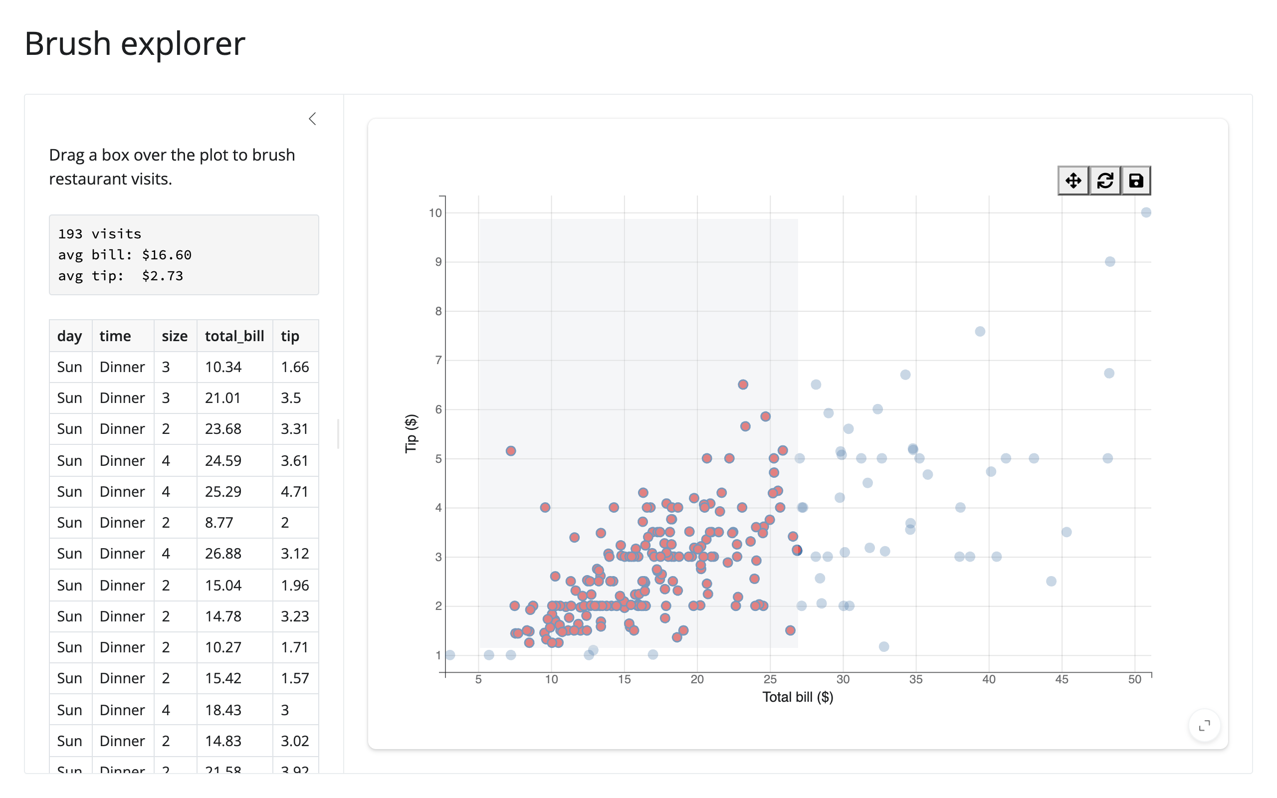
template_brush_explorer.py
A clean ~60-line starting point: brush a scatter plot of restaurant visits and read the selected rows into a summary and a table, both driven by selected_rows().
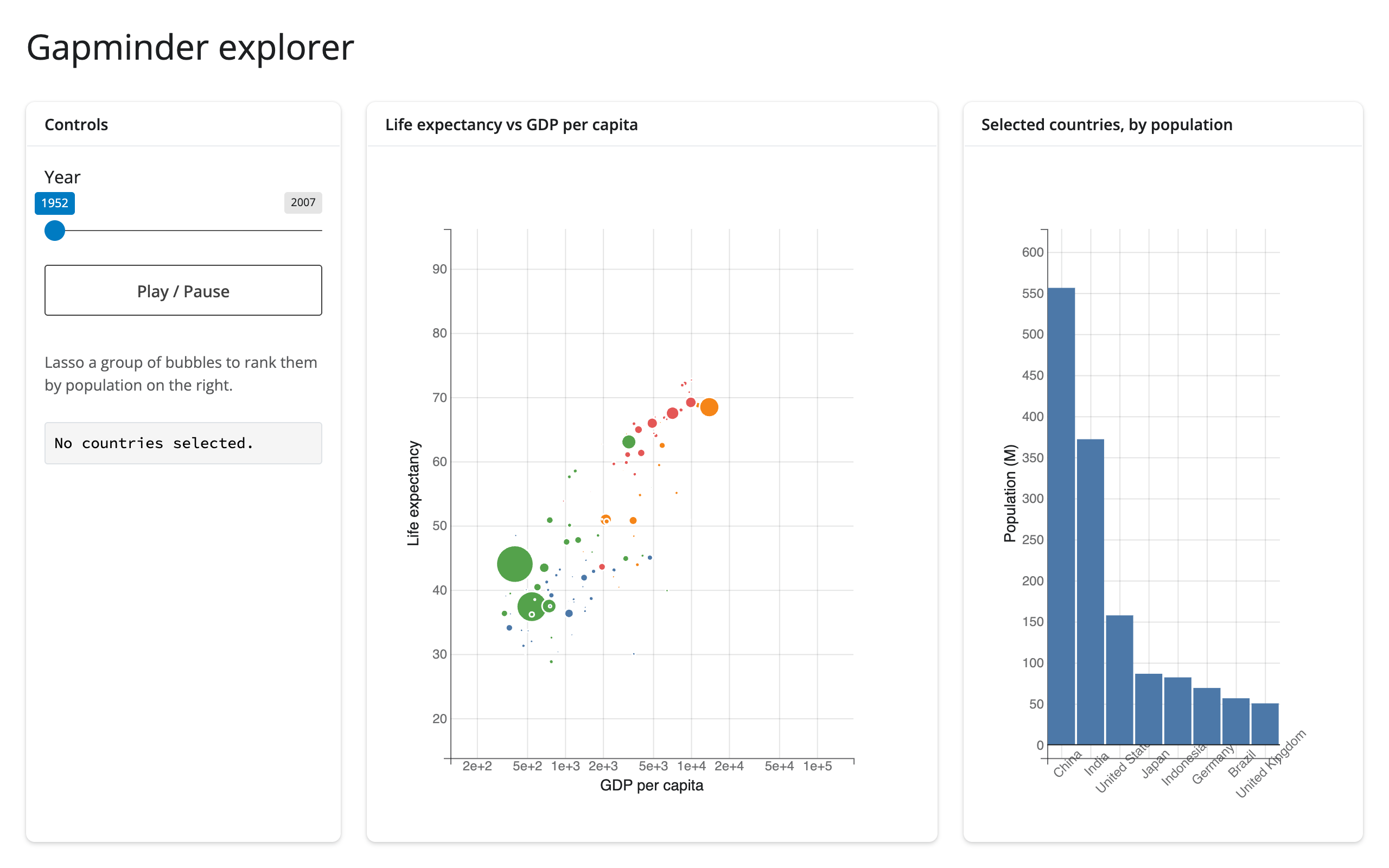
showcase_gapminder_explorer.py
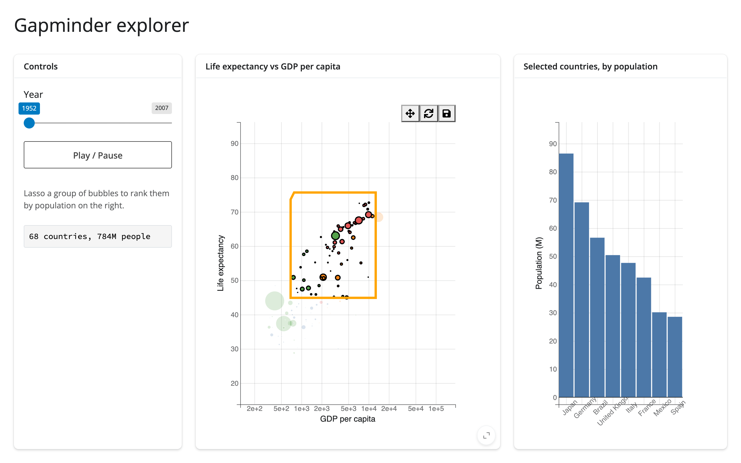
An animated Hans Rosling-style bubble chart with a play/pause autoplay loop, LassoSelector on the bubbles, and a ranked bar chart of the lassoed countries’ populations that updates in place (same hold_sync()/animation_ duration pattern as the quick-start animation). Exercises selected_rows() end to end: the lasso drives both the summary text and the second figure’s bars.
Learn more
- bqplot documentation and its example notebooks for the full mark/scale/axis API
- bqplot API reference for every mark type, scale type, and interaction
- Related guides in this roster: altair, plotly, itables, reactable