GeoViews

Cartopy-projected, tile-backed Bokeh maps from HoloViews/hvPlot elements – points, polygons, and choropleths that pan, zoom, and talk back to Python through the same stream recipe as HoloViews.

GeoViews is the geographic member of the HoloViz family (alongside HoloViews, hvPlot, Panel, and Datashader). It adds a crs (coordinate reference system) to HoloViews elements – gv.Points, gv.Polygons, gv.Path, gv.Image, gv.FilledContours, gv.WMTS tile layers, and Cartopy Features such as coastlines and borders – and reprojects them correctly when you overlay a web-map tile source or pick a real cartographic projection. It is maintained by the HoloViz team and is the natural choice when your data already lives in GeoPandas or xarray and you want the same declarative */+ composition and crossfilter story as plain HoloViews, just with geography done properly.

GeoViews maps render through the exact same @render_holoviews decorator as HoloViews/hvPlot – shinywidgets dispatches on the object’s module path, and geoviews.* classes route to the same Panel-to-Bokeh pipeline as holoviews.* ones. That means everything in the HoloViews guide carries over unchanged: layout and sizing (responsive=True, the fixed-height fillable=True trap), no reactive accessors (there’s no map.selected() to call), and the stream-subscriber recipe for turning clicks, box-selects, and viewport changes into Shiny reactive values. This guide assumes you’ve read the HoloViews guide and only covers what’s geographic: tile sources and projections, GeoPandas choropleths, hvPlot’s geo=True shortcut, and the specific coordinate-space behavior of each stream on a projected map.

Choose GeoViews when you want Bokeh-quality interactivity (pan, zoom, hover, linked streams) on a real map with a tile basemap or a non-Mercator projection, especially if you’re already using HoloViews/hvPlot elsewhere in the app or your data is a GeoDataFrame. For a point cloud in the tens or hundreds of thousands, prefer lonboard (WebGL/deck.gl) or GeoViews’ own Datashader rasterization (both covered below). For a Leaflet-style API with drawing tools and a more conventional “the map is the input” feel, see ipyleaflet or leafmap. For vector-tile styling with a Mapbox GL / MapLibre style spec, see maplibre.

hero

Installation

pip install 'shinywidgets[holoviews]' geoviews "cartopy<0.26"

There is no separate shinywidgets[geoviews] extra – GeoViews renders through the same holoviews extra (holoviews, panel, jupyter_bokeh>=4.1), the same way the HoloViews guide has you add hvplot yourself. Add geoviews and cartopy on top. The cartopy<0.26 pin matters: geoviews 1.15/1.16 raise KeyError: 'lon_0' from project_extents on cartopy 0.26 (fixed upstream in geoviews, not yet released as of this writing). This pass was verified with geoviews 1.16.0 and cartopy 0.25.0, where the pin is still necessary. Call hv.extension("bokeh") (or gv.extension("bokeh")) once per app, same as plain HoloViews, if you aren’t also importing hvplot.pandas.

Quick start

examples/01_quickstart.py29 lines

# A quick-start geoviews map: a tile basemap plus a scatter of real points,
# sized and colored by two more columns. Pan, zoom, and hover all come free.
import geoviews as gv
import holoviews as hv
import plotly.express as px
from shiny.express import ui

from shinywidgets import render_holoviews

hv.extension("bokeh")

carshare = px.data.carshare()

ui.page_opts(title="Montreal car-share stations", fillable=True)


@render_holoviews
def map():
    points = gv.Points(
        carshare, kdims=["centroid_lon", "centroid_lat"], vdims=["car_hours", "peak_hour"]
    ).opts(
        color="car_hours",
        cmap="viridis",
        size=8,
        colorbar=True,
        tools=["hover"],
        title="Car-share hours by station",
    )
    return (gv.tile_sources.OSM * points).opts(responsive=True)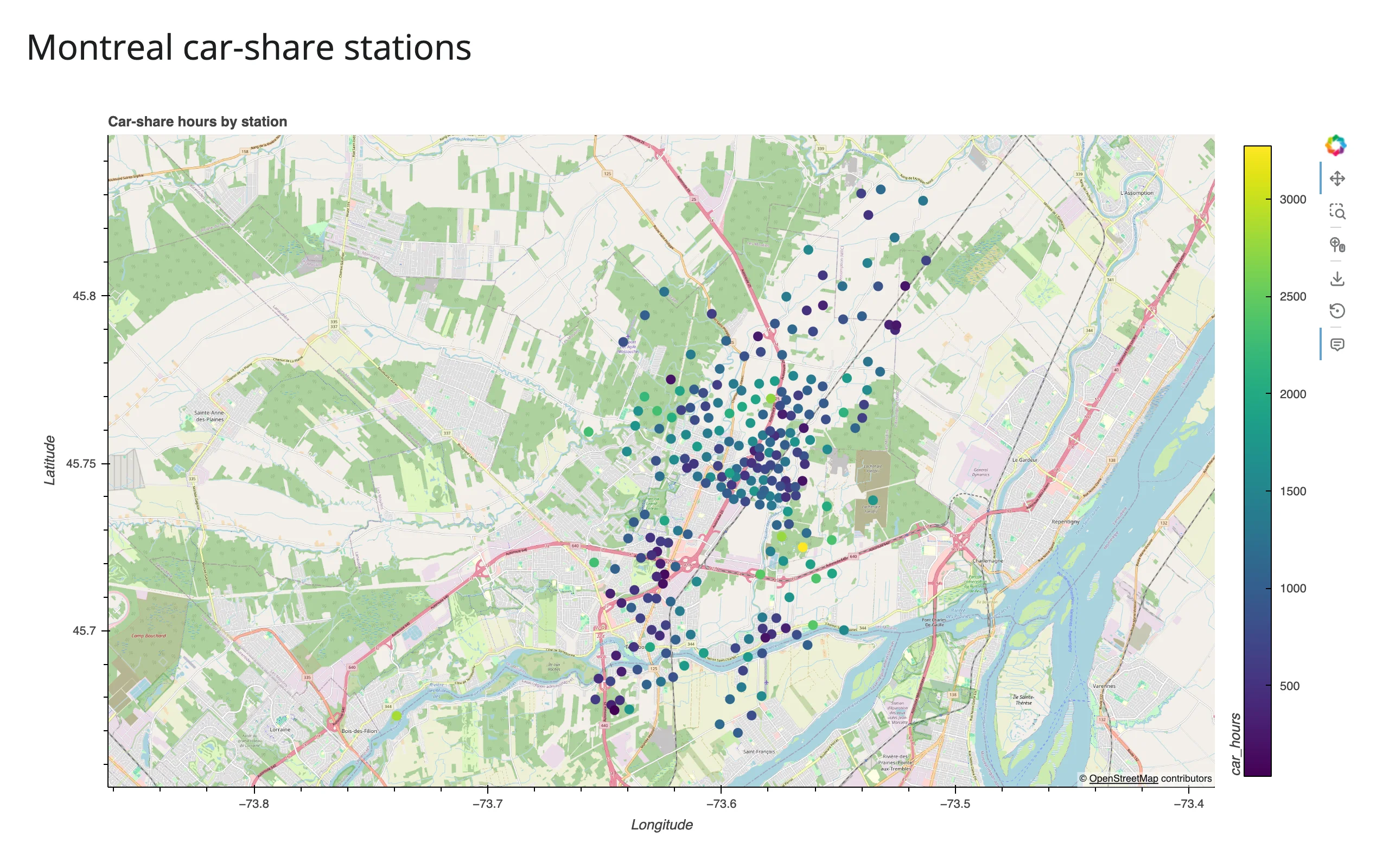

quick start

gv.tile_sources.OSM * points is the whole recipe: a tile layer overlaid (*) with a projected element. GeoViews ships 30+ built-in tile sources under gv.tile_sources – OSM, several Esri basemaps (EsriImagery, EsriWorldDarkGrayBase, EsriWorldShadedRelief, …), CartoDB, and more. Avoid CartoLight and CartoDark: they now return an “API key required” watermark tile with no key configured (verified today); Esri and OSM work without one. kdims are the point’s coordinate columns (lon, lat by default – GeoViews assumes PlateCarree, i.e. plain lon/lat, unless you pass crs=), and vdims are extra columns available to color=, size=, and hover tooltips.

What you can build

Polygons and choropleths from a real GeoDataFrame

examples/02_choropleth.py – a world population choropleth from Natural Earth’s 110m country polygons, built two ways: explicit gv.Polygons, and hvPlot’s one-line geo=True shortcut (downloads a small, public shapefile on first run):

examples/02_choropleth.py49 lines

# A world population choropleth from a real GeoDataFrame, two ways: explicit
# gv.Polygons, and hvPlot's one-line `geo=True` shortcut. Downloads Natural
# Earth's 110m country polygons (~200KB) on first run.
import geopandas as gpd
import geoviews as gv
import holoviews as hv
import hvplot.pandas  # noqa: F401
from shiny.express import ui

from shinywidgets import render_holoviews

hv.extension("bokeh")

NE_COUNTRIES = "https://naciscdn.org/naturalearth/110m/cultural/ne_110m_admin_0_countries.zip"
world = gpd.read_file(NE_COUNTRIES)
world = world[world.POP_EST > 0]  # a few disputed territories have no estimate

ui.page_opts(title="World population (Natural Earth, 110m)", fillable=True)

with ui.layout_columns():
    with ui.card(full_screen=True):
        ui.card_header("gv.Polygons, explicit")

        @render_holoviews
        def explicit():
            return gv.Polygons(
                world, vdims=["NAME", "POP_EST"]
            ).opts(
                color="POP_EST",
                cmap="viridis",
                logz=True,
                colorbar=True,
                tools=["hover"],
                responsive=True,
            )

    with ui.card(full_screen=True):
        ui.card_header("hvPlot, geo=True")

        @render_holoviews
        def shortcut():
            return world.hvplot(
                c="POP_EST",
                geo=True,
                cmap="viridis",
                logz=True,
                hover_cols=["NAME"],
                responsive=True,
            )

choropleth: explicit vs. hvPlot shortcut

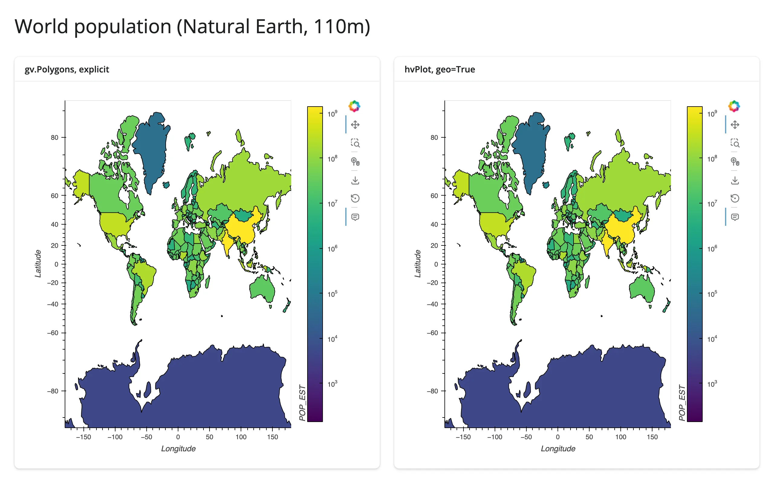
Both render identically. gv.Polygons(gdf, vdims=[...]) reads the GeoDataFrame’s geometry column directly – no manual lon/lat extraction – and gdf.hvplot(geo=True, ...) is the hvPlot equivalent for anyone who’d rather stay in the .hvplot accessor style from the HoloViews guide. logz=True is doing a lot of work here: population is extremely right-skewed, and a linear color scale would make everything but China and India look identical.

Projections: Web Mercator vs. the real thing

examples/03_projections.py – the same 300 scattered points, once with a Web Mercator tile basemap (the default whenever tiles are involved), once with projection=ccrs.Robinson() and no tiles:

examples/03_projections.py44 lines

# Web Mercator (the default, needed for tile basemaps) vs. a real cartographic
# projection. Swapping `projection=` reshapes the coastlines and repositions
# every point -- there is no "zoom into a Robinson map" the way there is with
# tiles, since tiles only exist pre-rendered in Web Mercator.
import cartopy.crs as ccrs
import geoviews as gv
import geoviews.feature as gf
import holoviews as hv
import numpy as np
from shiny.express import ui

from shinywidgets import render_holoviews

hv.extension("bokeh")

rng = np.random.default_rng(0)
# A few hundred points scattered near shipping lanes, for visual texture
lons = rng.uniform(-180, 180, 300)
lats = rng.uniform(-60, 75, 300)

ui.page_opts(title="Web Mercator vs. a real projection", fillable=True)

with ui.layout_columns():
    with ui.card(full_screen=True):
        ui.card_header("Default: Web Mercator, with tiles")

        @render_holoviews
        def mercator():
            pts = gv.Points((lons, lats)).opts(color="firebrick", size=3, alpha=0.6)
            return (gv.tile_sources.OSM * pts).opts(responsive=True)

    with ui.card(full_screen=True):
        ui.card_header("projection=ccrs.Robinson(), no tiles")

        @render_holoviews
        def robinson():
            pts = gv.Points((lons, lats)).opts(color="firebrick", size=3, alpha=0.6)
            overlay = gf.coastline * gf.borders * pts
            return overlay.opts(
                "Points",
                responsive=True,
            ).opts(
                projection=ccrs.Robinson(), global_extent=True, title="Robinson"
            )

Web Mercator vs. Robinson

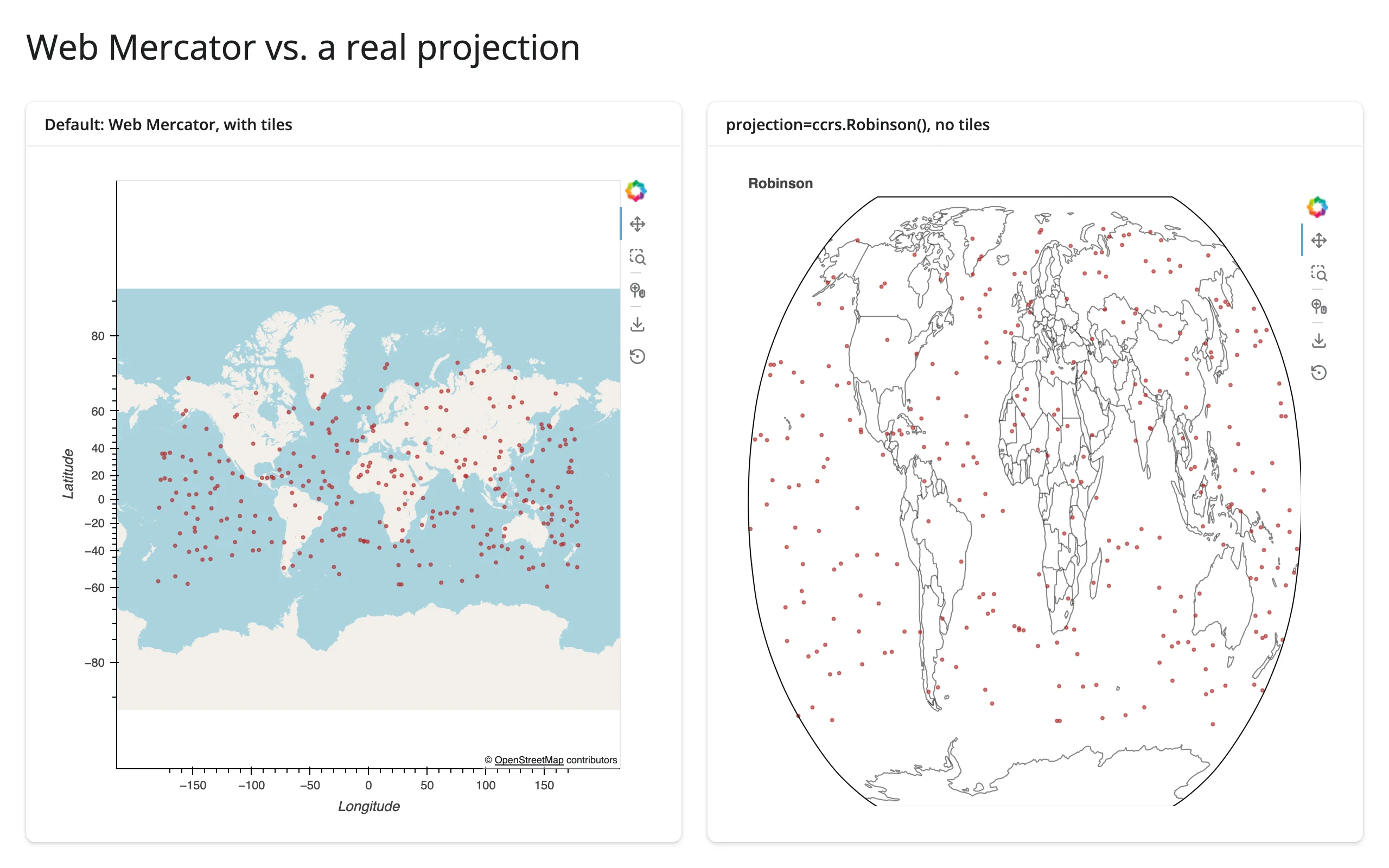
What actually changes: the axes go from lon/lat degrees to the projection’s own linear units, every point and coastline is reprojected (look at how much Alaska and Antarctica’s apparent shape changes), and the tile basemap disappears – tiles are pre-rendered raster images that only exist in Web Mercator, so a non-Mercator projection= has nothing to overlay them onto. global_extent=True tells GeoViews to frame the whole globe instead of auto-ranging to just the data’s bounding box, which matters once there’s no tile layer providing an implicit extent. gf.coastline, gf.borders, gf.ocean, gf.land, and gf.lakes are Cartopy Natural Earth features that download on first use (see Gotchas) and project with everything else automatically.

Paths

gv.Path works the same way as gv.Points – a sequence of lon/lat vertices that reprojects with the rest of the overlay. It isn’t demonstrated as a separate example here since there’s nothing geography-specific about it beyond what gv.Points/gv.Polygons already show; see the HoloViews elements reference for the full element list.

Scaling up: rasterizing points

examples/08_rasterize_scale.py – the same 200,000 points sent two ways: raw coordinates, and pre-aggregated into a fixed-size image with hvPlot’s rasterize=True:

examples/08_rasterize_scale.py44 lines

# 200,000 points sent as raw coordinates (left) vs. rasterized to a fixed-size
# image on the server before it ever reaches the browser (right). Both pan and
# zoom the same way, but the rasterized version re-aggregates per view instead
# of shipping every point -- see ../datashader/guide.md for the full story.
import geoviews as gv
import holoviews as hv
import hvplot.pandas  # noqa: F401
import numpy as np
import pandas as pd
from shiny.express import ui

from shinywidgets import render_holoviews

hv.extension("bokeh")

rng = np.random.default_rng(0)
n = 200_000
cities = np.array([(-74, 41), (-0.1, 51.5), (139, 35.7), (28, -26), (151, -34)])
center = cities[rng.integers(0, len(cities), n)]
points = pd.DataFrame(
    center + rng.normal(0, 3.0, (n, 2)), columns=["lon", "lat"]
)

ui.page_opts(title="200,000 points: raw vs. rasterized", fillable=True)

with ui.layout_columns():
    with ui.card(full_screen=True):
        ui.card_header("Raw gv.Points (every coordinate shipped)")

        @render_holoviews
        def raw():
            return (gv.tile_sources.EsriWorldDarkGrayBase * gv.Points(points, kdims=["lon", "lat"]).opts(
                size=2, alpha=0.1, color="cyan"
            )).opts(responsive=True)

    with ui.card(full_screen=True):
        ui.card_header("hvPlot rasterize=True (fixed-size image)")

        @render_holoviews
        def rasterized():
            return points.hvplot.points(
                "lon", "lat", geo=True, rasterize=True, dynspread=True,
                cmap="fire", tiles="EsriWorldDarkGrayBase", responsive=True,
            )

raw vs. rasterized

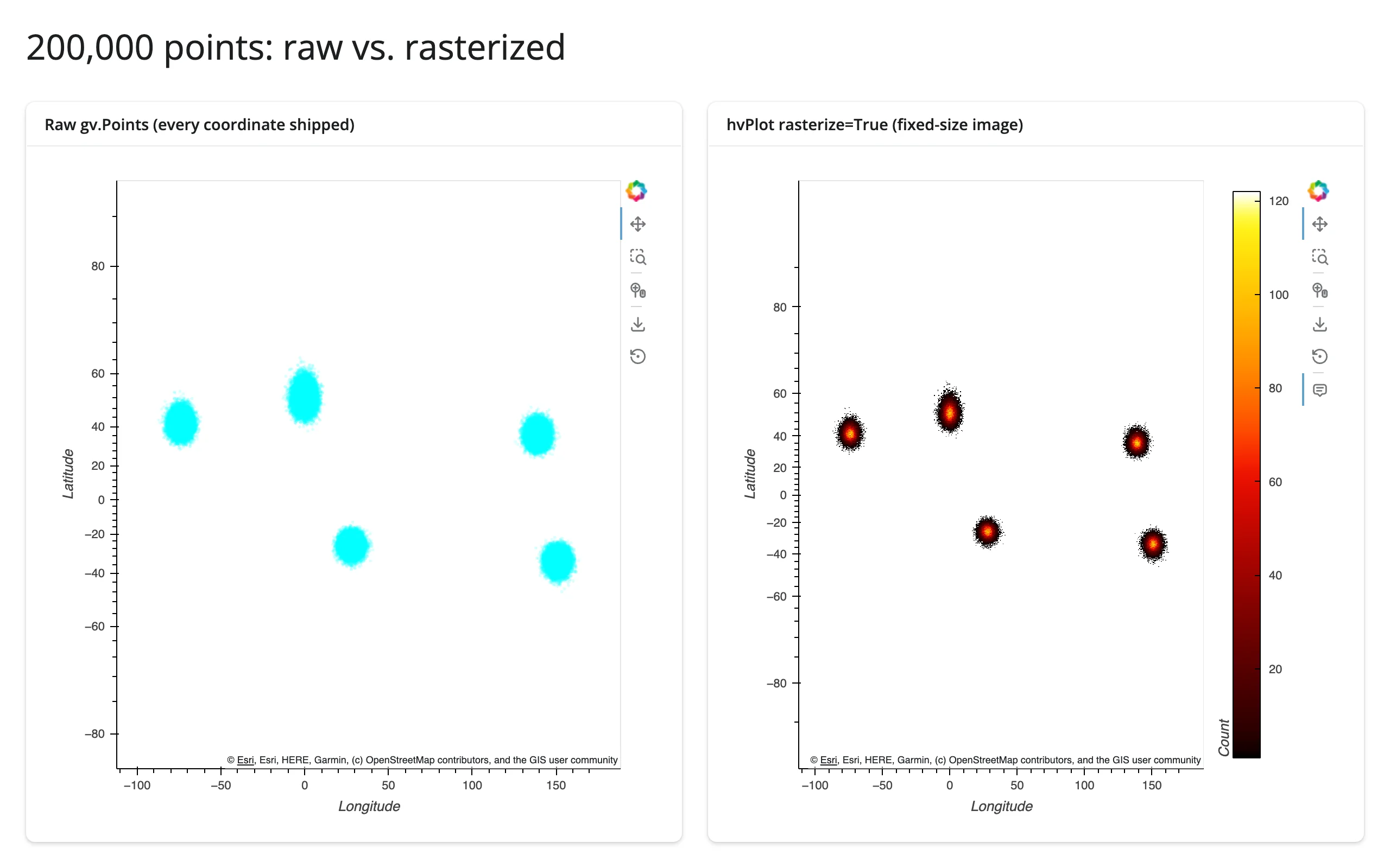
The left panel ships all 200,000 (lon, lat) pairs to the browser as plain glyph data – every pan/zoom redraws the same fixed set of circles, and the overplotted blob tells you nothing about density. The right panel’s rasterize=True runs Datashader on the server: it bins every point into a small, fixed number of pixels server-side and sends a single image, so the payload size doesn’t grow with the point count and you get an actual density field (the color ramp) instead of a solid blob. dynspread=True widens isolated pixels by a point or two so sparse areas stay visible. This is the same mechanism as rasterize()/datashade() in plain HoloViews – see the HoloViews guide and the Datashader guide for the full picture (rate of re-aggregation, dynspread vs. spread, categorical aggregation, etc.).

When to hand off: a few thousand points render fine as plain gv.Points (the earthquake examples later in this guide use ~6,000 with no issue). Tens of thousands to millions of points is GeoViews’ and Datashader’s sweet spot if you want server-side aggregation (heatmap-style density, no picking of individual points). If you need every point to stay pickable/selectable at that scale with GPU-smooth pan and zoom, prefer lonboard (deck.gl/WebGL) instead – its accessors (selected(), clicked()) also give you per-point interactivity that a rasterized image can’t. For local raster files (GeoTIFF/COG) rather than point clouds, see localtileserver.

Reacting to user interaction

Same story as plain HoloViews: render_holoviews has no reactive accessors. GeoViews elements use HoloViews’ own streams (hv.streams.Tap, BoundsXY, RangeXY, …), and the recipe is identical – subscribe to the stream inside the render function and set a reactive.Value from the callback. Read the HoloViews guide’s recipe first; this section only covers what’s different about coordinates on a projected map.

The coordinate-space rule that matters here: streams attached to a GeoViews element report their values in that element’s own coordinates – lon/lat by default – regardless of what CRS the plot actually draws in underneath a tile basemap (Web Mercator). This is true for Tap, BoundsXY, and RangeXY: GeoViews reprojects the browser’s reported pixel range back to the source element’s crs before your subscriber ever sees it. Verified directly: a RangeXY reading the rendered Bokeh model’s raw x_range/y_range is in Web Mercator meters (e.g. -8211102.97), but the exact same pan/zoom reported through hv.streams.RangeXY(source=points) arrives in plain lon/lat (e.g. -73.74). You never need holoviews.util.transform.easting_northing_to_lon_lat for reading stream values back – only if you set a static xlim=/ylim= option on a tiled plot (see Gotchas).

Pattern: click a feature for details

examples/04_tap_detail.py – hv.streams.Tap on a gv.Points layer, same as the HoloViews guide’s Tap example:

examples/04_tap_detail.py48 lines

# Click a station on the map to see its details. hv.streams.Tap reports the
# click in data coordinates (lon/lat), even though the map draws in Web
# Mercator -- geoviews un-projects it for you. Same recipe as the holoviews
# guide's Tap example; see ../holoviews/guide.md#the-recipe.
import geoviews as gv
import holoviews as hv
import plotly.express as px
from shiny import reactive
from shiny.express import render, ui

from shinywidgets import render_holoviews

hv.extension("bokeh")

carshare = px.data.carshare()
tap_xy = reactive.value(None)

ui.page_opts(title="Click a station for details", fillable=True)

with ui.layout_columns():
    with ui.card(full_screen=True):

        @render_holoviews
        def map():
            points = gv.Points(
                carshare, kdims=["centroid_lon", "centroid_lat"], vdims=["car_hours"]
            ).opts(color="car_hours", cmap="viridis", size=8, tools=["tap", "hover"])
            hv.streams.Tap(source=points).add_subscriber(
                lambda x, y: tap_xy.set((x, y))
            )
            return (gv.tile_sources.OSM * points).opts(responsive=True)

    with ui.card():
        ui.card_header("Nearest station")

        @render.ui
        def detail():
            xy = tap_xy()
            if xy is None:
                return ui.p("Click a station on the map.", class_="text-muted")
            x, y = xy
            dist = (carshare.centroid_lon - x) ** 2 + (carshare.centroid_lat - y) ** 2
            row = carshare.loc[dist.idxmin()]
            return ui.TagList(
                ui.h5(f"{row.car_hours:.0f} car-hours"),
                ui.p(f"Peak hour: {row.peak_hour:.0f}:00"),
                ui.p(f"{row.centroid_lat:.4f}, {row.centroid_lon:.4f}", class_="text-muted"),
            )

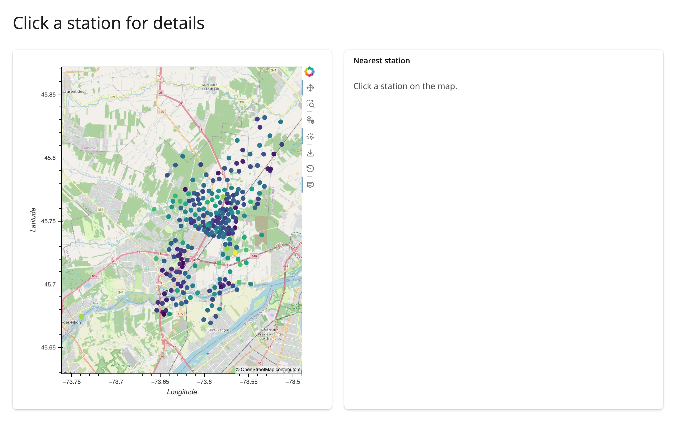
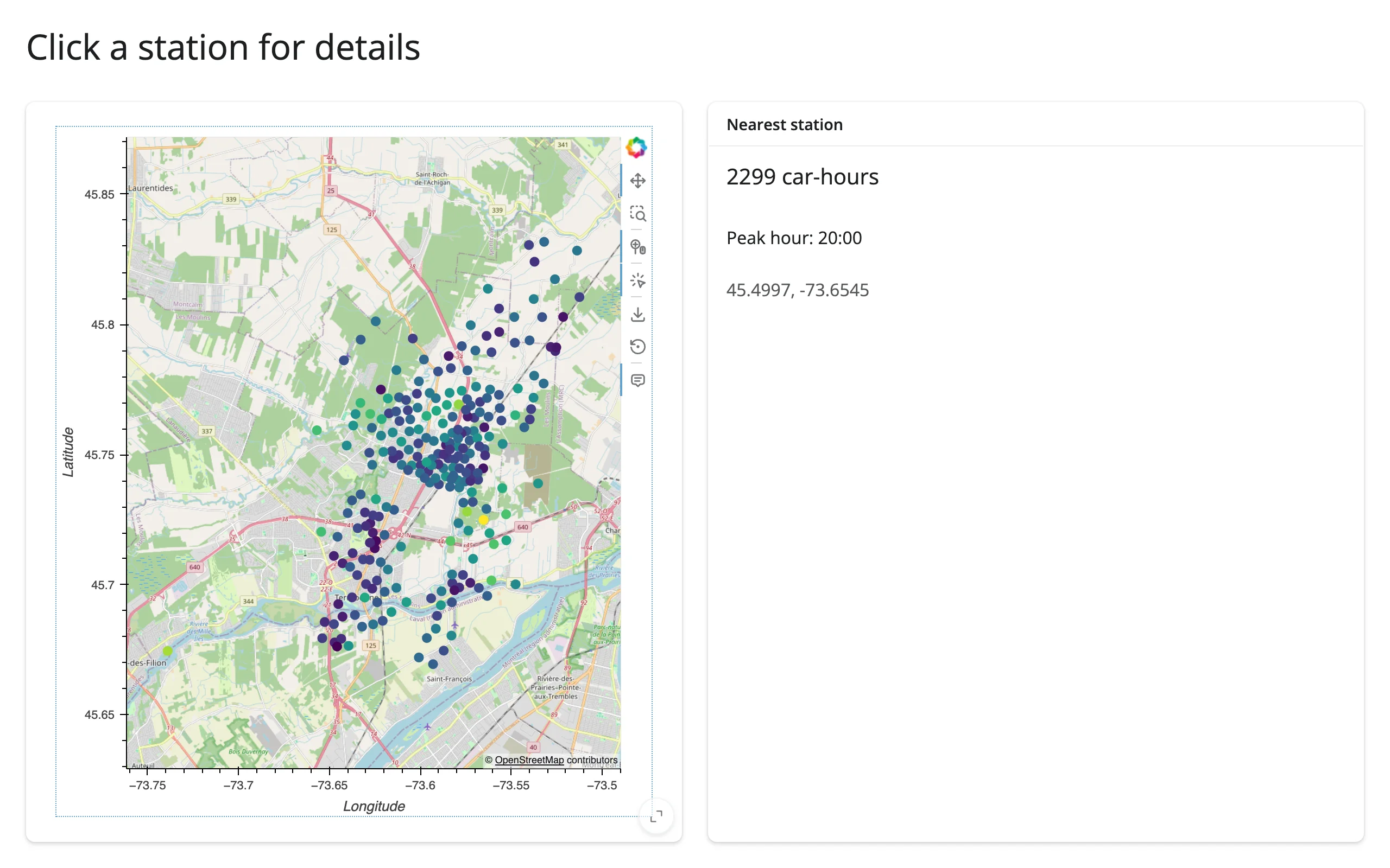
Tap reports the click location regardless of whether it landed exactly on a point glyph, so “nearest row by squared distance” (same pattern as the HoloViews guide) is the right lookup on the Shiny side.

Pattern: box-select to filter a table

examples/05_boundsxy_table.py – hv.streams.BoundsXY reports the dragged rectangle, already in lon/lat, so it tests directly against a plain pandas DataFrame with no reprojection:

examples/05_boundsxy_table.py50 lines

# Box-select stations on the map to filter a table below it. BoundsXY reports
# the dragged rectangle in lon/lat, so the same bounds test a plain pandas
# DataFrame -- no re-projection needed on the Shiny side.
import geoviews as gv
import holoviews as hv
import plotly.express as px
from shiny import reactive
from shiny.express import render, ui

from shinywidgets import render_holoviews

hv.extension("bokeh")

carshare = px.data.carshare()
bounds_val = reactive.value(None)

ui.page_opts(title="Box-select stations to filter a table", fillable=True)

with ui.card(full_screen=True):

    @render_holoviews
    def map():
        points = gv.Points(
            carshare, kdims=["centroid_lon", "centroid_lat"], vdims=["car_hours"]
        ).opts(
            color="car_hours",
            cmap="viridis",
            size=8,
            tools=["box_select"],
            active_tools=["box_select"],
        )
        hv.streams.BoundsXY(source=points).add_subscriber(
            lambda bounds: bounds_val.set(bounds)
        )
        return (gv.tile_sources.OSM * points).opts(responsive=True)


with ui.card():
    ui.card_header("Stations in view")

    @render.data_frame
    def selected():
        b = bounds_val()
        if b is None:
            return carshare.iloc[:0]
        x0, y0, x1, y1 = b
        sel = carshare[
            carshare.centroid_lon.between(x0, x1) & carshare.centroid_lat.between(y0, y1)
        ]
        return render.DataGrid(sel.round(2), height="220px")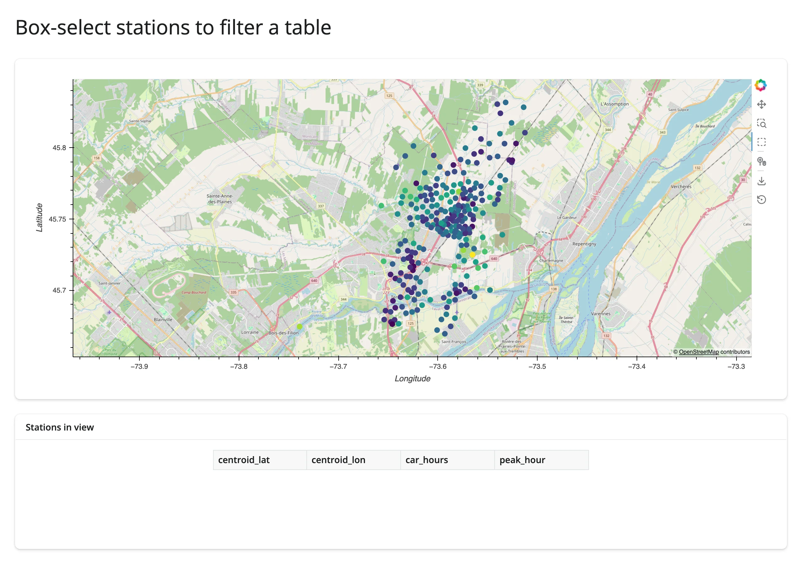

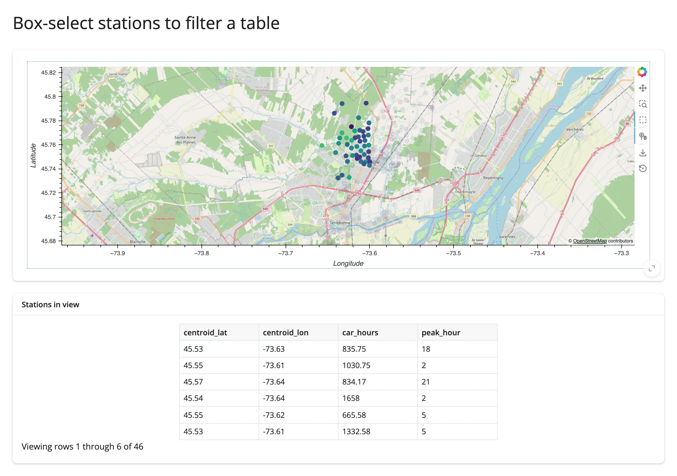
Note this example keeps the map output full width (not in a ui.layout_columns() column next to the table) as a layout preference – box-select itself works fine in a narrower column too, see Gotchas.

Pattern: viewport drives summary stats

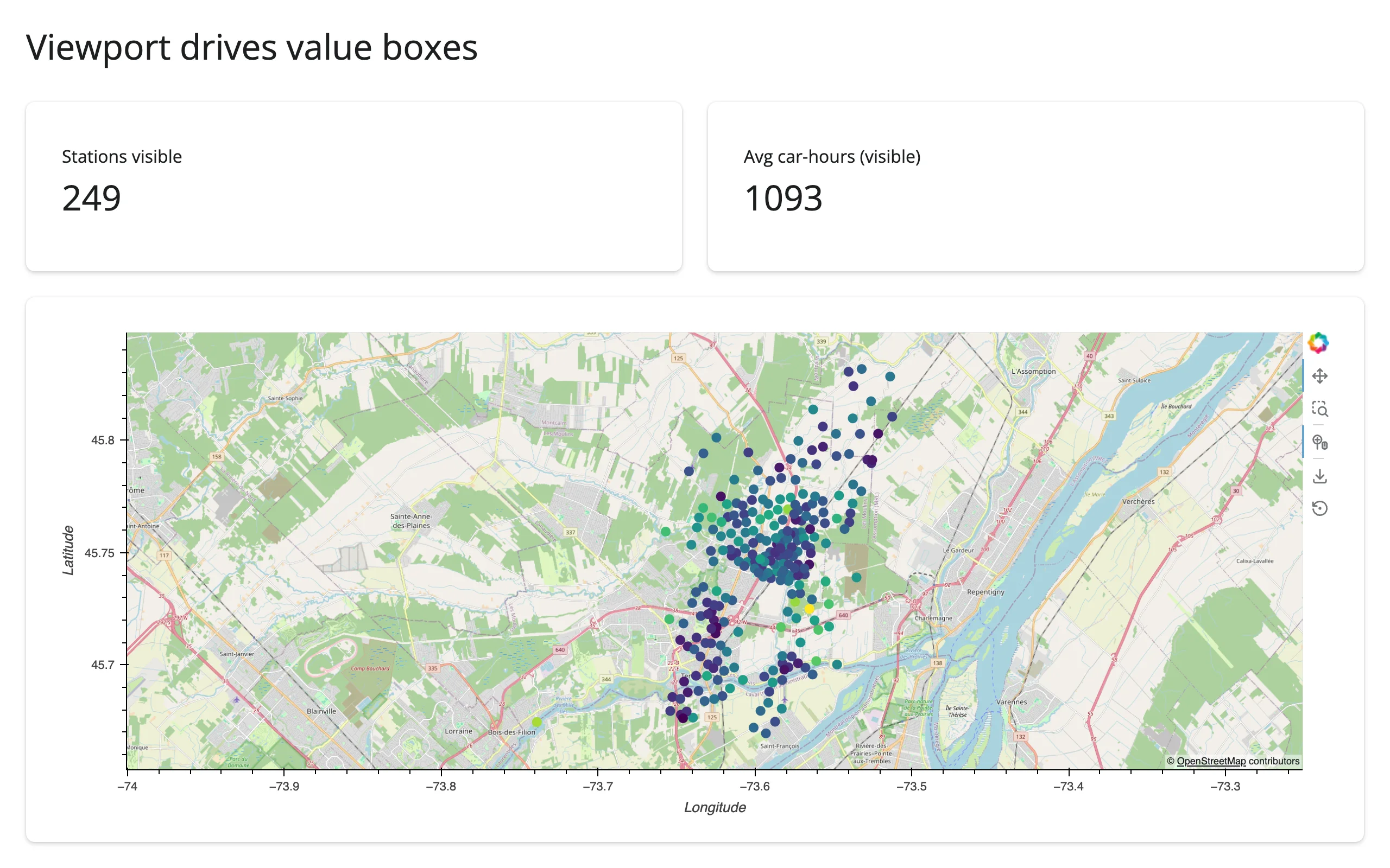
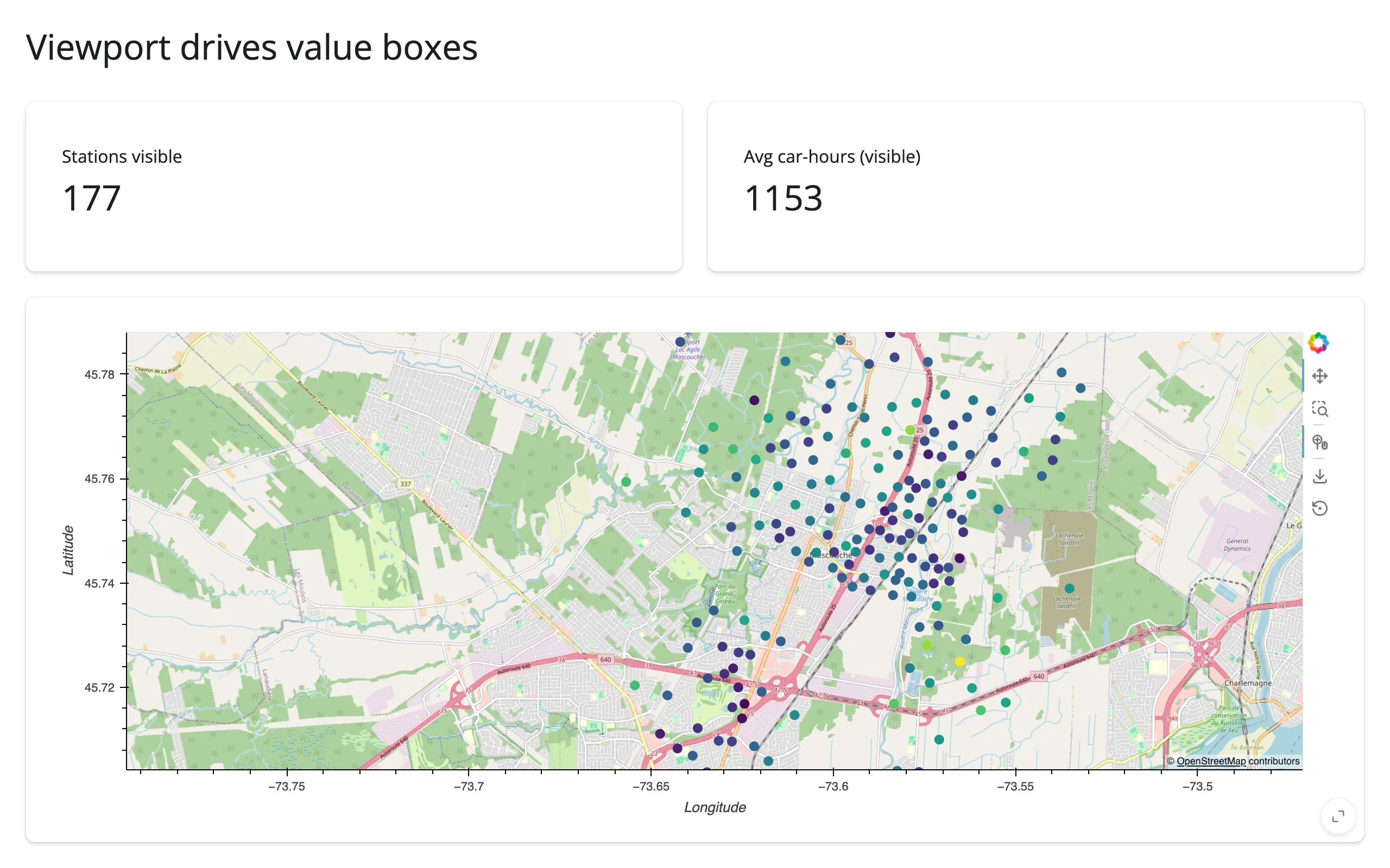
hv.streams.RangeXY reports the current pan/zoom extent continuously (on every frame of a drag or scroll-zoom, not just once per gesture like BoundsXY/Tap). Store the stream’s own range tuple, never a counter – reactive.Value.set() then skips invalidating readers on repeated, unchanged reports, so a long scroll-zoom doesn’t recompute anything after the range stops moving (examples/06_rangexy_viewport.py):

examples/06_rangexy_viewport.py66 lines

# The visible viewport drives two value boxes. hv.streams.RangeXY reports the
# current x_range/y_range in the *source element's* coordinates -- lon/lat for
# a geoviews element, same as BoundsXY/Tap -- even though the plot itself
# draws in Web Mercator underneath the tiles.
#
# Store the stream's own (idempotent) range tuple, never a counter: a stream
# that fires on every animation frame of a zoom, combined with an
# ever-different subscriber value, causes a render loop (see Gotchas).
import geoviews as gv
import holoviews as hv
import plotly.express as px
from shiny import reactive
from shiny.express import render, ui

from shinywidgets import render_holoviews

hv.extension("bokeh")

carshare = px.data.carshare()
range_val = reactive.value(None)

ui.page_opts(title="Viewport drives value boxes", fillable=True)

with ui.layout_columns(fill=False):
    with ui.value_box():
        "Stations visible"

        @render.text
        def n_visible():
            return str(len(visible()))

    with ui.value_box():
        "Avg car-hours (visible)"

        @render.text
        def avg_hours():
            v = visible()
            return f"{v.car_hours.mean():.0f}" if len(v) else "-"


with ui.card(full_screen=True):

    @render_holoviews
    def map():
        points = gv.Points(
            carshare, kdims=["centroid_lon", "centroid_lat"], vdims=["car_hours"]
        ).opts(
            color="car_hours", cmap="viridis", size=8,
            tools=["wheel_zoom"], active_tools=["wheel_zoom"],
        )
        hv.streams.RangeXY(source=points).add_subscriber(
            lambda x_range, y_range: range_val.set((x_range, y_range))
        )
        return (gv.tile_sources.OSM * points).opts(responsive=True)


@reactive.calc
def visible():
    r = range_val()
    if r is None or None in r[0] or None in r[1]:
        return carshare
    (lon0, lon1), (lat0, lat1) = r
    return carshare[
        carshare.centroid_lon.between(lon0, lon1)
        & carshare.centroid_lat.between(lat0, lat1)
    ]

Beyond streams: reactive_read

Same as the HoloViews guide: reactive_read() doesn’t apply to streams or GeoViews elements themselves (they’re param.Parameterized objects, not ipywidgets traits). reactive_read(x.widget, "trait") (or the equivalent x.read("trait")) still technically works on the rendered BokehModel, but there’s rarely a reason to reach for it here – render_holoviews has no accessors, so .read()’s only job is that trait fallback, and a BokehModel’s traits don’t reflect anything map-specific.

Rate limiting

rate_policy/rate_delay do nothing for this recipe, same caveat as the HoloViews guide. In practice Tap and BoundsXY each fire once per gesture, so there’s nothing to throttle. RangeXY is the one stream here that fires repeatedly (every frame of a drag-pan or scroll-zoom) – store its own value idempotently (as in the example above) rather than rate-limiting it, so repeated frames with the same range are a no-op instead of extra traffic.

Updating the widget from Python

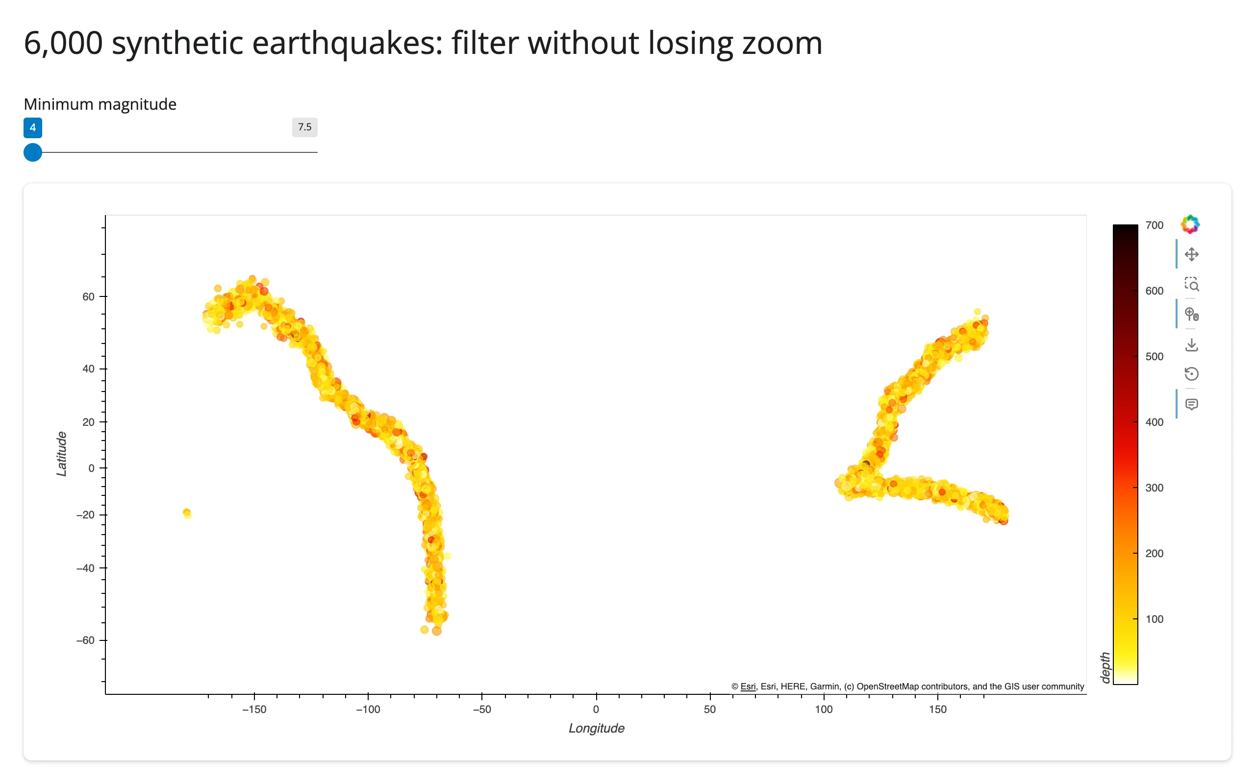
Identical mechanism to the HoloViews guide: driving a hv.DynamicMap with a hv.streams.Pipe updates the existing Bokeh model in place (same comm, same JS-side glyphs), which preserves the user’s pan/zoom; re-rendering from a plain Shiny input read rebuilds the plot and resets the view. examples/07_inplace_filter.py shows the geographic case: a magnitude slider filters 6,000 synthetic earthquakes without losing the zoom.

examples/07_inplace_filter.py64 lines

# A magnitude slider filters 6,000 synthetic earthquakes without losing the
# user's zoom: the slider drives a holoviews.streams.Pipe, not a re-render.
# This is the same recipe as ../holoviews/guide.md's Pipe example -- see
# "Updating the widget from Python" there for the re-render-vs-in-place
# contrast in full. Synthetic data here is about *scale* (see "Performance
# with large point sets" in the guide text); the belt shape is just for
# visual plausibility.
import geoviews as gv
import holoviews as hv
import numpy as np
from shiny import reactive
from shiny.express import input, ui

from shinywidgets import render_holoviews

hv.extension("bokeh")

rng = np.random.default_rng(1)
# Two separate belts (Americas, Asia-Pacific) -- kept apart so linear
# interpolation never cuts straight across the Pacific at the antimeridian.
BELTS = [
    np.array([(-70, -55), (-71, -33), (-75, -10), (-80, 5), (-90, 15),
               (-100, 20), (-120, 35), (-125, 48), (-150, 60), (-170, 55)]),
    np.array([(170, 52), (150, 45), (140, 35), (130, 30), (125, 10),
               (120, 0), (110, -8), (130, -8), (150, -10), (170, -15), (178, -20)]),
]
lons, lats = [], []
for belt in BELTS:
    for a, b in zip(belt[:-1], belt[1:]):
        t = rng.uniform(0, 1, 320)
        seg = a * (1 - t[:, None]) + b * t[:, None] + rng.normal(0, 1.5, (320, 2))
        lons.append(seg[:, 0])
        lats.append(seg[:, 1])
lons, lats = np.concatenate(lons), np.concatenate(lats)
n = len(lons)
mag = rng.exponential(0.6, n).clip(0, 4) + 4.0  # Gutenberg-Richter-ish tail
depth = rng.gamma(2.0, 60, n).clip(0, 700)
quakes = {"lon": lons, "lat": lats, "mag": mag, "depth": depth}

ui.page_opts(title="6,000 synthetic earthquakes: filter without losing zoom", fillable=True)
ui.input_slider("min_mag", "Minimum magnitude", min=4.0, max=7.5, value=4.0, step=0.5)

pipe = hv.streams.Pipe(data=quakes)


def quake_points(data):
    return gv.Points(data, kdims=["lon", "lat"], vdims=["mag", "depth"]).opts(
        color="depth", cmap="fire_r", size=hv.dim("mag") * 1.5, alpha=0.6,
        colorbar=True, tools=["hover", "wheel_zoom"], active_tools=["wheel_zoom"],
    )


with ui.card(full_screen=True):

    @render_holoviews
    def map():
        dmap = hv.DynamicMap(quake_points, streams=[pipe])
        return (gv.tile_sources.EsriWorldDarkGrayBase * dmap).opts(responsive=True)


@reactive.effect
def _():
    mask = mag >= input.min_mag()
    pipe.send({"lon": lons[mask], "lat": lats[mask], "mag": mag[mask], "depth": depth[mask]})

Zoomed into Japan, then the slider moved from 4.0 to 5.5:

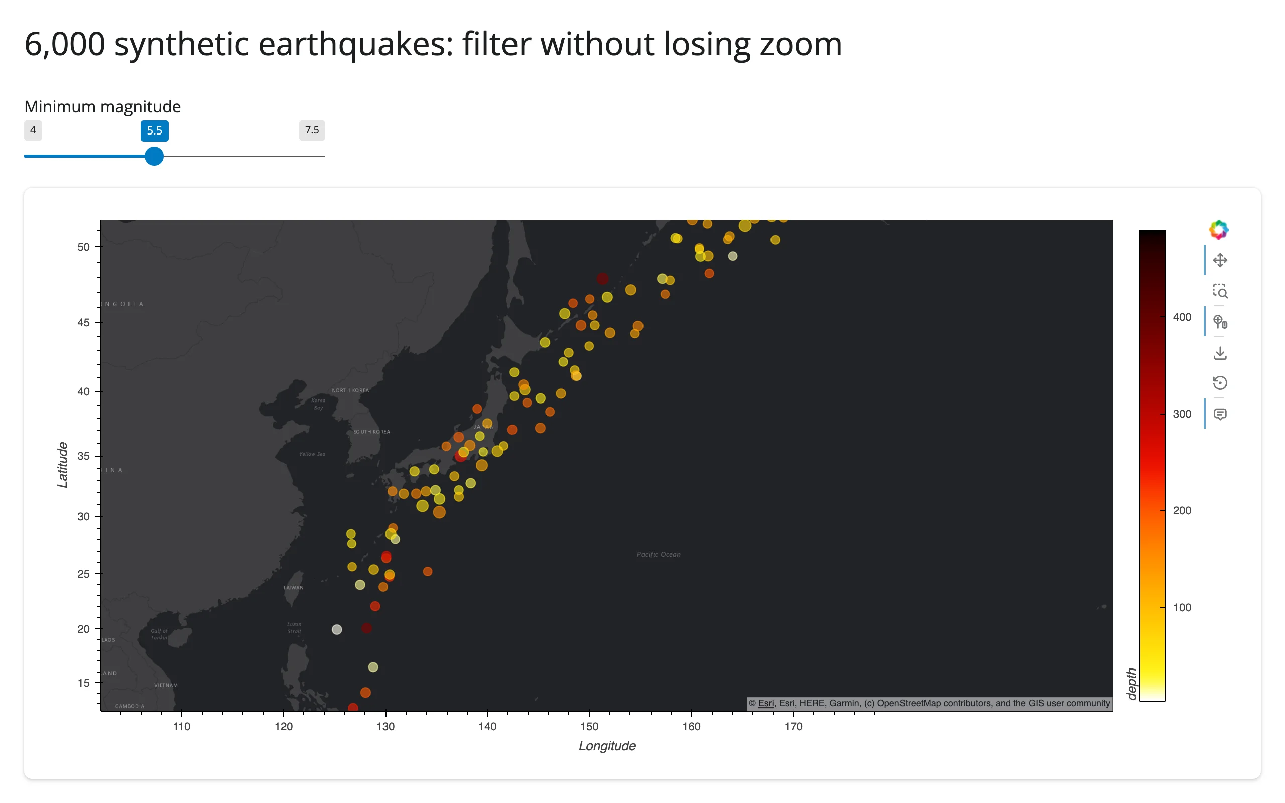
The viewport (axis range) is identical in both screenshots; only the points changed. Important: attach Tap/BoundsXY/RangeXY to the DynamicMap object itself (hv.streams.Tap(source=dmap)), not to the element returned from inside its callback function. A fresh stream instance created on every callback invocation never gets wired to the live plot’s JS callbacks – only the very first invocation’s streams do. This bit the showcase gallery app during development; see Gotchas.

Coordinating multiple views

Three complete, gesture-verified patterns – building on the streams above:

1. Click → nearest feature → detail card – examples/04_tap_detail.py, shown above under Reacting to user interaction.
2. Box-select → filtered table – examples/05_boundsxy_table.py, shown above.
3. Viewport (pan/zoom) → summary stats – examples/06_rangexy_viewport.py, shown above, the same pattern as the HoloViews guide’s zoom-range example. Store the stream’s own range tuple, not a counter or anything else that changes on every call – good practice regardless of the coordinate space, since reactive.Value.set() only re-runs readers when the range actually changed.

The gallery showcase (below) combines all three (slider → in-place filter, box-select → value boxes and a table, click → detail card) in one dashboard.

Large data

GeoViews’ large-data mode is rasterize=True (via hvPlot or HoloViews’ rasterize()), which runs Datashader on the server and sends one fixed-size image instead of every point – summarize on the server. Scaling up: rasterizing points above measures this directly: 200,000 raw gv.Points ship every coordinate and overplot into a solid blob, while the rasterized version sends a single image whose payload doesn’t grow with point count. Plain (non-rasterized) gv.Points/gv.Polygons render fine into the low thousands (this guide’s earthquake examples use ~6,000); past that, rasterize, or switch to lonboard if individual points need to stay pickable. See the Large data & performance article for how this compares to the other two approaches.

Layout and sizing

Nothing GeoViews-specific beyond the HoloViews guide’s section: responsive=True fills the container, a fixed output_widget(..., height=) needs fillable=True alongside it, and full_screen=True on the card works normally. One thing worth calling out here because maps make it obvious: a colorbar=True legend and a tile attribution string both live inside the same Bokeh figure, so they share whatever width/height the plot gets – there’s no separate layout slot for them.

Gotchas and limitations

Verified on current main (shiny 1.9.0, geoviews 1.16.0, holoviews 1.23.2, hvplot 0.12.2, cartopy 0.25.0, panel 1.10.0, bokeh 3.10.1, geopandas 1.2.0, jupyter_bokeh 4.1.0). Everything in the HoloViews guide’s Gotchas applies here too (the sidebar/second-output link_selections claims there were retracted after a follow-up investigation; RangeXY’s old re-render-loop bug is fixed – see below); this list covers what’s additionally true for GeoViews.

• A BoundsXY (box-select) stream silently never fires below _500-650px~ – retracted, test-methodology artifact, not a bug. An earlier revision of this guide reported box-select failing on a narrow responsive canvas. A follow-up investigation found the real mechanism: Bokeh’s BoxSelectTool only starts a selection when the mousedown lands inside the plot’s data frame, not its fixed-pixel y-axis label margin (~49px). A drag computed as a fraction of the canvas’s full bounding rect clears that margin comfortably on a wide canvas (a few percent of the width) but lands inside the margin once the canvas is narrow enough (the same 49px is now ten-plus percent of the width) – confirmed down to a 222px-wide canvas with a drag computed from the plot’s actual frame bounds instead, which selects correctly at any width tested. This is a property of how a synthetic test drag is computed, not of the canvas width itself: a real user dragging with a mouse naturally starts inside the visible plot area and is unaffected. No code change or layout workaround is needed; examples/05_boundsxy_table.py keeps its map output full-width purely as a layout preference, not because narrower columns are broken.
• Attach streams to the DynamicMap, not to the element its callback returns. hv.streams.Tap(source=pts) created inside a DynamicMap callback function creates a fresh, disconnected stream object on every call; only a stream attached to the DynamicMap itself (hv.streams.Tap(source=dmap), built once per render) stays wired to the live plot. Verified: the broken form renders fine and shows no error, but the subscriber is simply never invoked.
• RangeXY no longer risks a re-render loop – shinywidgets runs widget coercion under reactive.isolate(), so a stream subscriber’s reactive reads can’t register the in-progress render as a dependent (see the HoloViews guide’s Gotchas for the mechanism). Still store the stream’s own range tuple, not a counter, as this guide’s viewport example does: it’s idempotent once the user stops interacting, so reactive.Value.set() skips invalidating readers on repeats, which avoids pointless recomputation even though it’s no longer needed to avoid a crash. Verified on current main: a multi-step scroll-zoom produced zero RuntimeError: BokehModel was closed tracebacks in the server log.
• Stream values come back in the element’s native coordinates (lon/lat by default), not the tile layer’s Web Mercator – for Tap and BoundsXY and RangeXY. Only a static .opts(xlim=..., ylim=...) on an overlay that includes tiles needs Mercator meters (convert with holoviews.util.transform.lon_lat_to_easting_northing); reading values back out of any stream does not. This is worth being explicit about because it’s easy to assume (incorrectly) that everything involving tiles needs that conversion.
• A non-Mercator projection= drops any tile layer silently (no error – the overlay just renders without a basemap). Tiles are Web-Mercator-only raster images; there is no server-side reprojection path for them. Verified with projection=ccrs.Robinson() plus gv.tile_sources.OSM in the overlay.
• .opts() on gv.tile_sources.* and gv.feature.* mutates the shared module-level object in place. Style with .opts(..., clone=True) or one session’s styling leaks into every other session and output that reuses the same tile/feature object (this follows from normal Python object-identity semantics, not something shinywidgets-specific, but it’s an easy trap the first time you reach for gv.tile_sources.OSM.opts(alpha=0.5)).
• CartoLight/CartoDark tiles now require an API key and render an “API key required” watermark instead (verified today, both as a plain gv.tile_sources.CartoDark and via hvPlot’s tiles="CartoDark"). Use an Esri preset or OSM.
• gv.feature.* (coastline, borders, ocean, land, lakes) downloads Natural Earth shapefiles on first use, synchronously, inside the render call. Offline servers should pre-warm Cartopy’s data cache; the first request that needs a feature will otherwise stall.
• geoviews 1.15/1.16 require cartopy<0.26 (KeyError: 'lon_0' from project_extents otherwise, reproduced directly with a bare gv.Points, no shinywidgets involved). The fix is merged upstream but unreleased as of this writing.
• An empty element (e.g. a req()-guarded selection that filters everything out) collapses the map’s extent to a near-zero-degree box, which then floods the tile server with requests at the deepest zoom level. Guard with req(...) on the input that could produce an empty frame, same as any other shinywidgets output.

Gallery candidates

gallery/template_city_map.py (template)

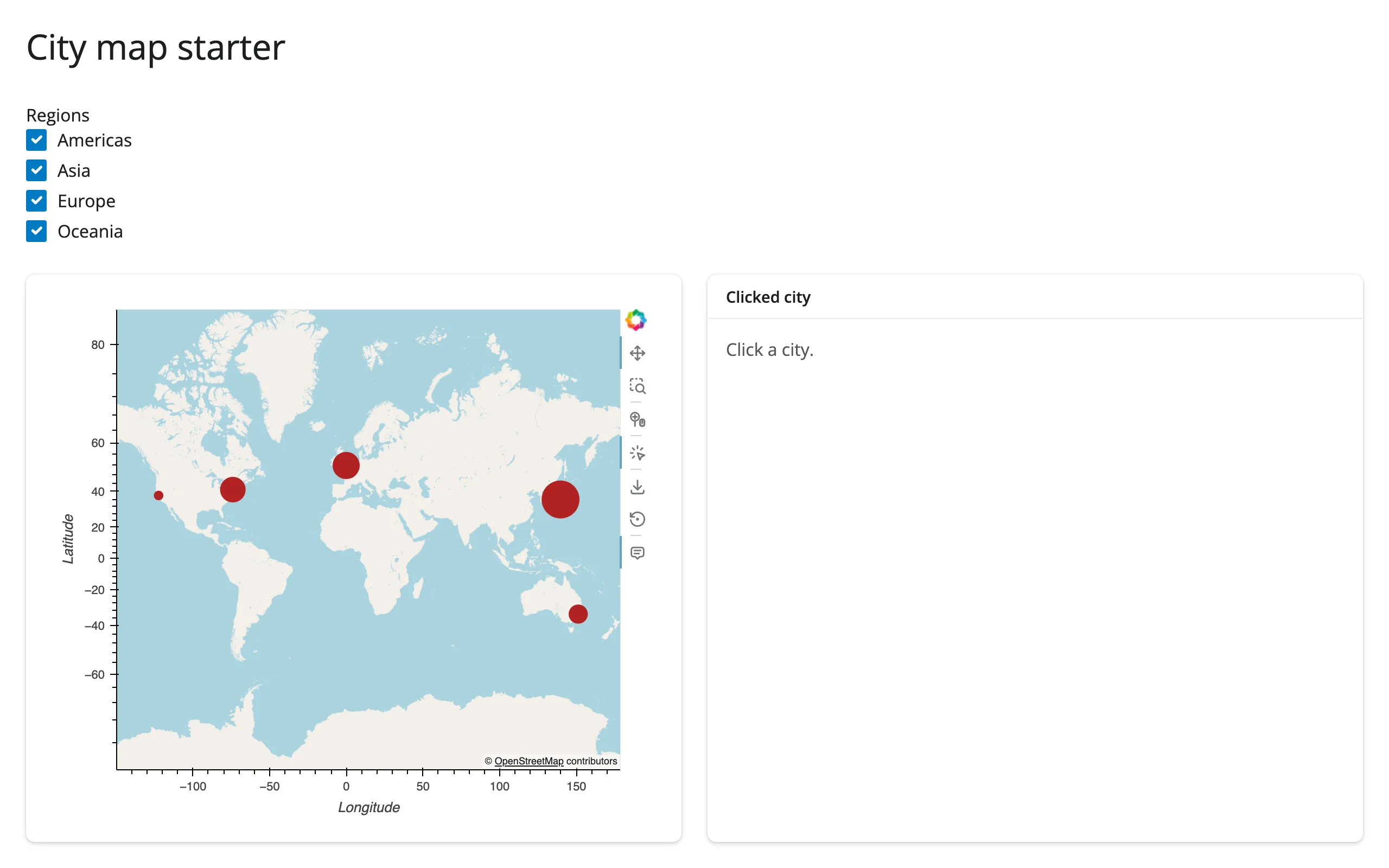
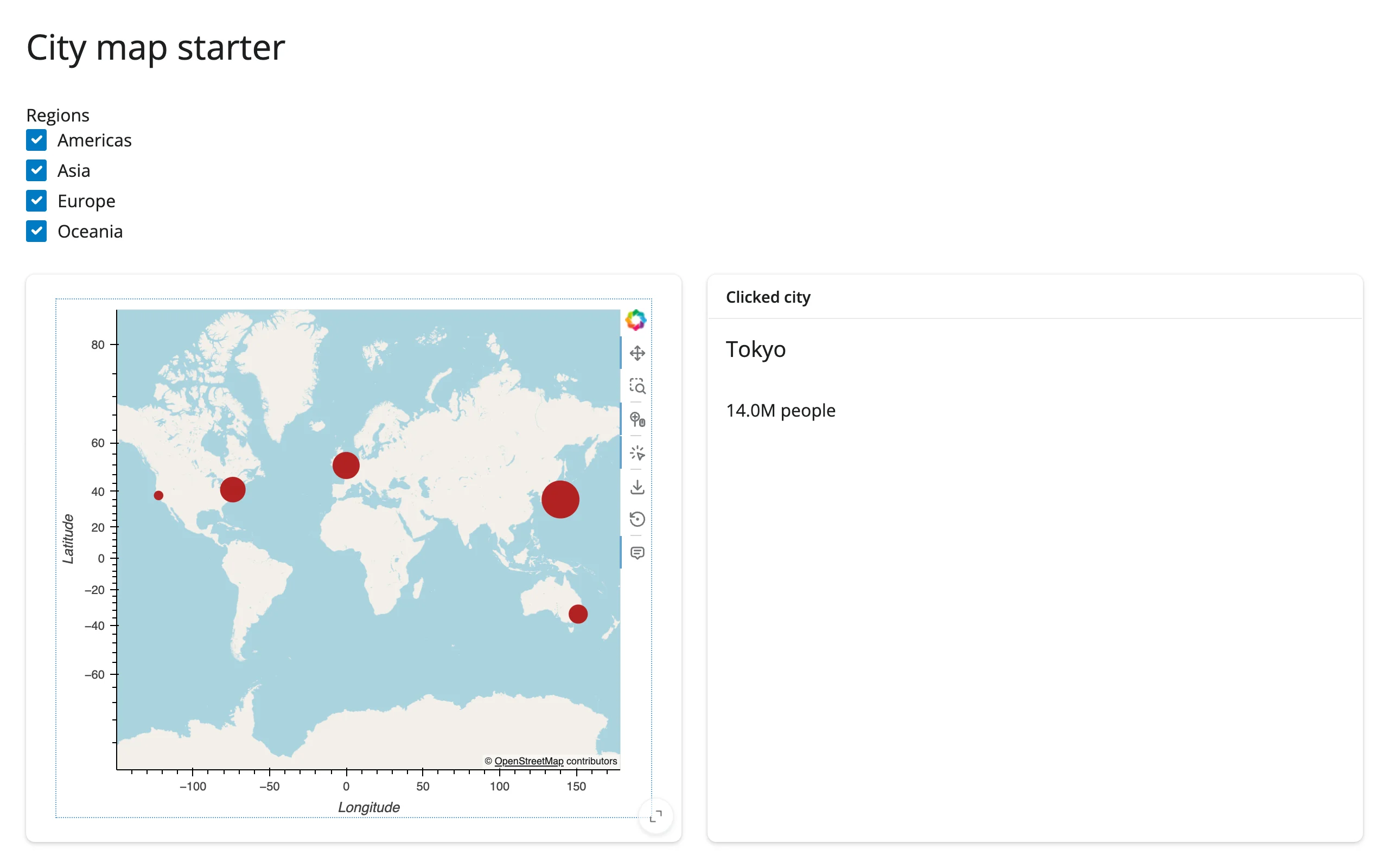
A minimal, adaptable starting point: six world cities on an OSM basemap, sized by population, with a region checkbox filter and click-for-detail. Swap in your own DataFrame and tile source.

gallery/showcase_quake_explorer.py (showcase)

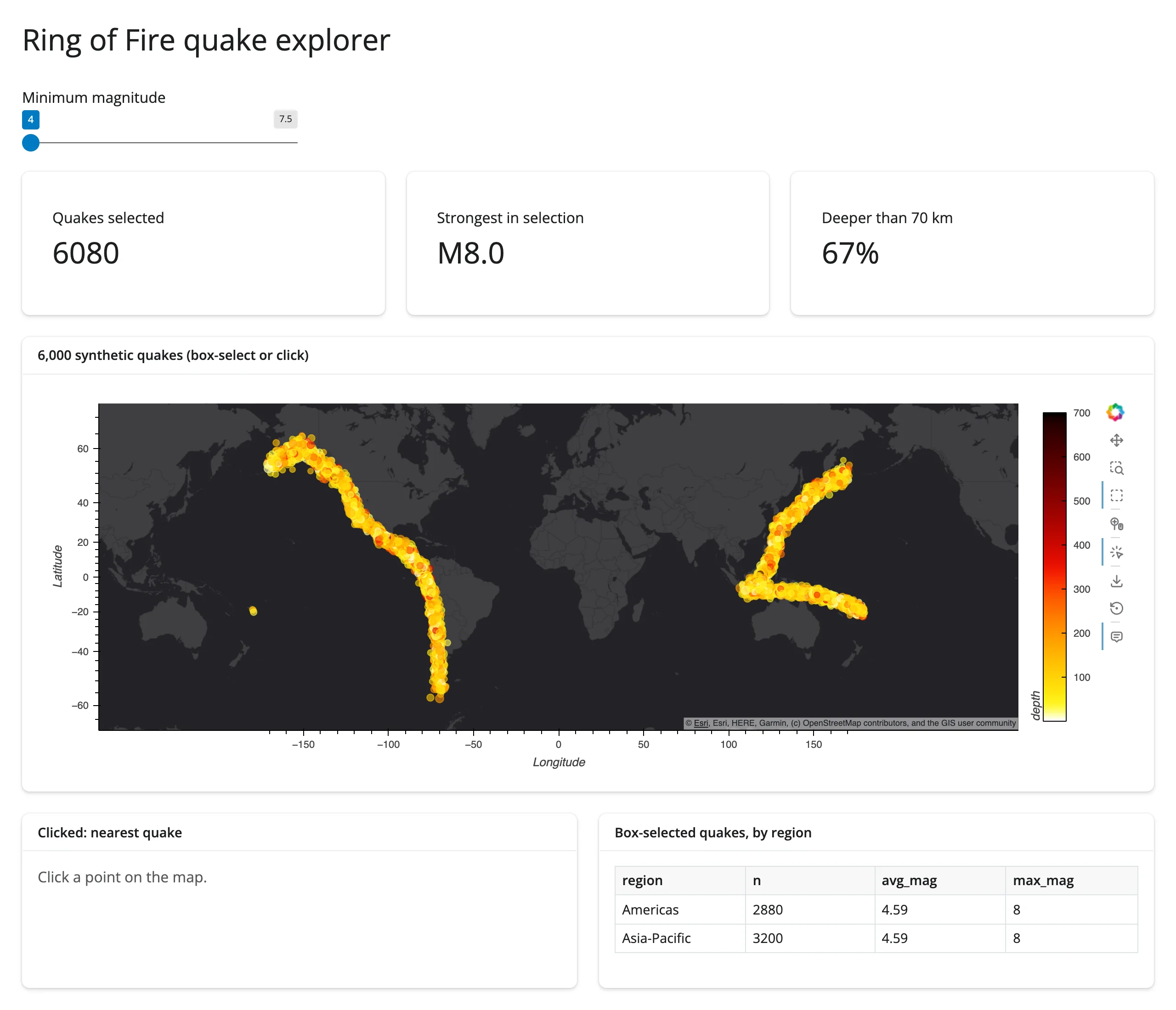
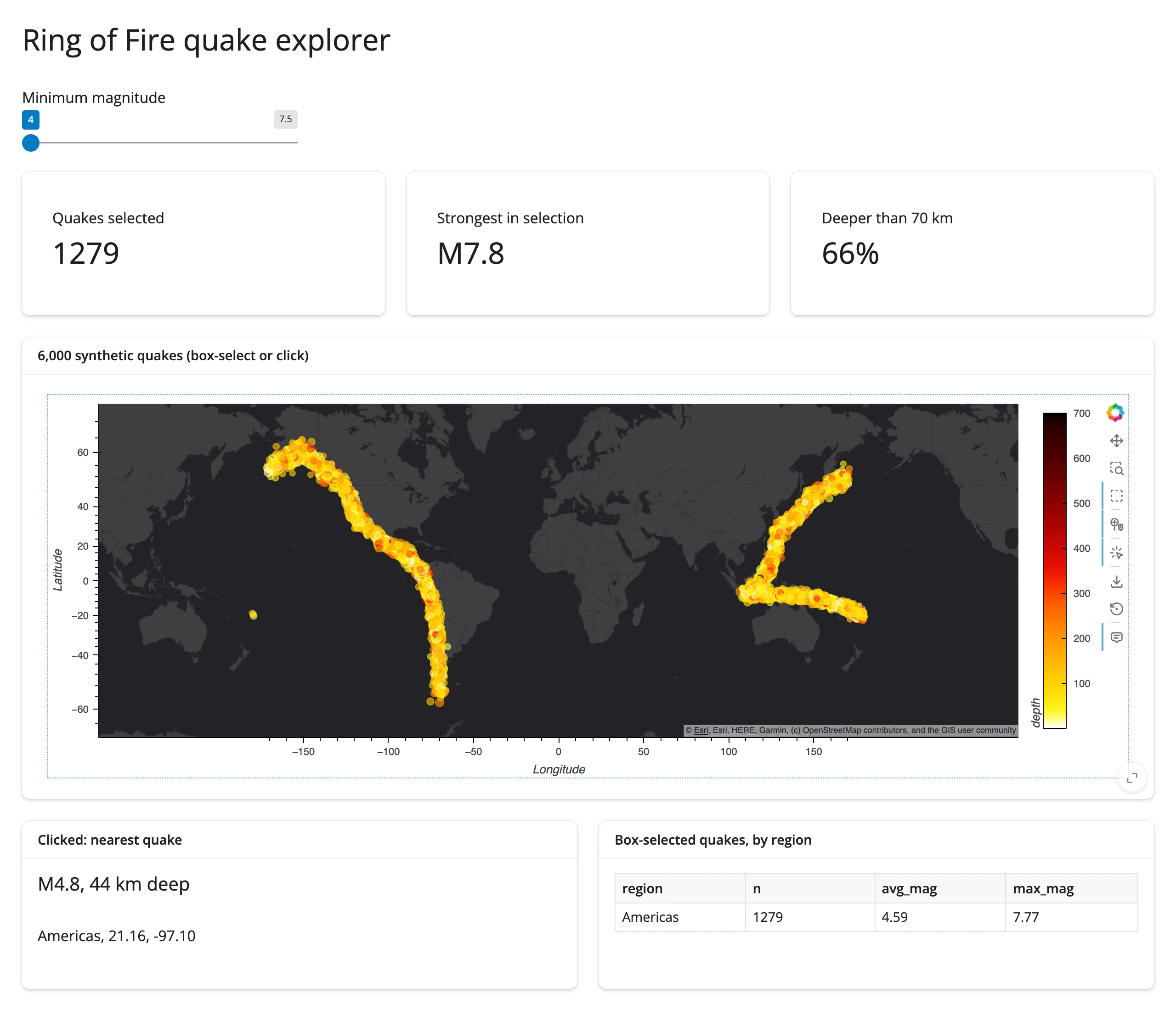
“Ring of Fire quake explorer” – 6,000 synthetic earthquakes on a dark Esri basemap, combining every pattern in this guide: a magnitude slider drives an in-place Pipe update (preserves zoom), box-select drives three value boxes and a by-region table via BoundsXY, and a click drives a detail card via Tap. The map is kept full-width as a layout preference, not a workaround – see Gotchas.

Learn more

• GeoViews documentation – element types, projections, gallery
• GeoViews user guide: Projecting data
• Cartopy CRS reference – all available ccrs.* projections
• Related guides in this roster: holoviews (read this first), datashader, bokeh, lonboard, ipyleaflet, leafmap, maplibre, localtileserver