Matplotlib

Turn any matplotlib figure into a live, zoomable, clickable widget without leaving Python.

Matplotlib is the foundation of the Python plotting ecosystem: pandas’ .plot(), seaborn, statsmodels, scikit-learn’s *Display classes, mplfinance, and many others all draw onto a matplotlib Figure under the hood. It’s been developed by a large open-source community since 2003 and is uniquely good at precise, static, publication-quality graphics with total control over every element.

@render_matplotlib renders a figure as a live ipympl widget instead of a static image. The decorated function may return a Figure, an Axes, or an ipympl.backend_nbagg.Canvas directly, which covers anything built on matplotlib. Shinywidgets fits the figure to its container (or keeps its figsize with an explicit height), keeps re-renders from leaking pyplot figures across sessions, and surfaces draw-time errors as a normal output error instead of killing the session. On top of that, three reactive accessors – clicked(), picked(), and limits() – read what the user does with the figure, much like reading a Shiny input.

Reach for @render_matplotlib when the plot should respond to the user: panning and zooming, clicking to inspect a point, or updating a line in place without redrawing the whole figure. Reach for Shiny’s own @render.plot when a picture is enough – it’s cheaper (a PNG per render), the safest choice for many concurrent users, and it applies tight layout and closes its figure automatically. If you draw with the grammar-of-graphics style instead of matplotlib’s imperative API, see the plotnine guide, which renders through this same ipympl engine and shares its clicked() and limits() accessors.

Installation

pip install 'shinywidgets[matplotlib]'

This installs matplotlib and ipympl, the widget backend that @render_matplotlib renders through.

Quick start

Decorate a function that builds and returns a Figure. Build it with matplotlib.figure.Figure() directly (or plt.subplots(), closed automatically when rendered) rather than relying on pyplot’s implicit current figure – see Gotchas.

examples/01_quickstart.py19 lines

from matplotlib.cbook import get_sample_data
from matplotlib.figure import Figure
from shiny.express import ui
from shinywidgets import render_matplotlib

ui.page_opts(fillable=True)

# Google's daily closing price from its 2004 IPO through the 2008 crash,
# bundled with matplotlib as sample data
goog = get_sample_data("goog.npz")["price_data"]


@render_matplotlib
def plot():
    fig = Figure(layout="constrained")
    ax = fig.subplots()
    ax.plot(goog["date"], goog["close"])
    ax.set_ylabel("Close ($)")
    return fig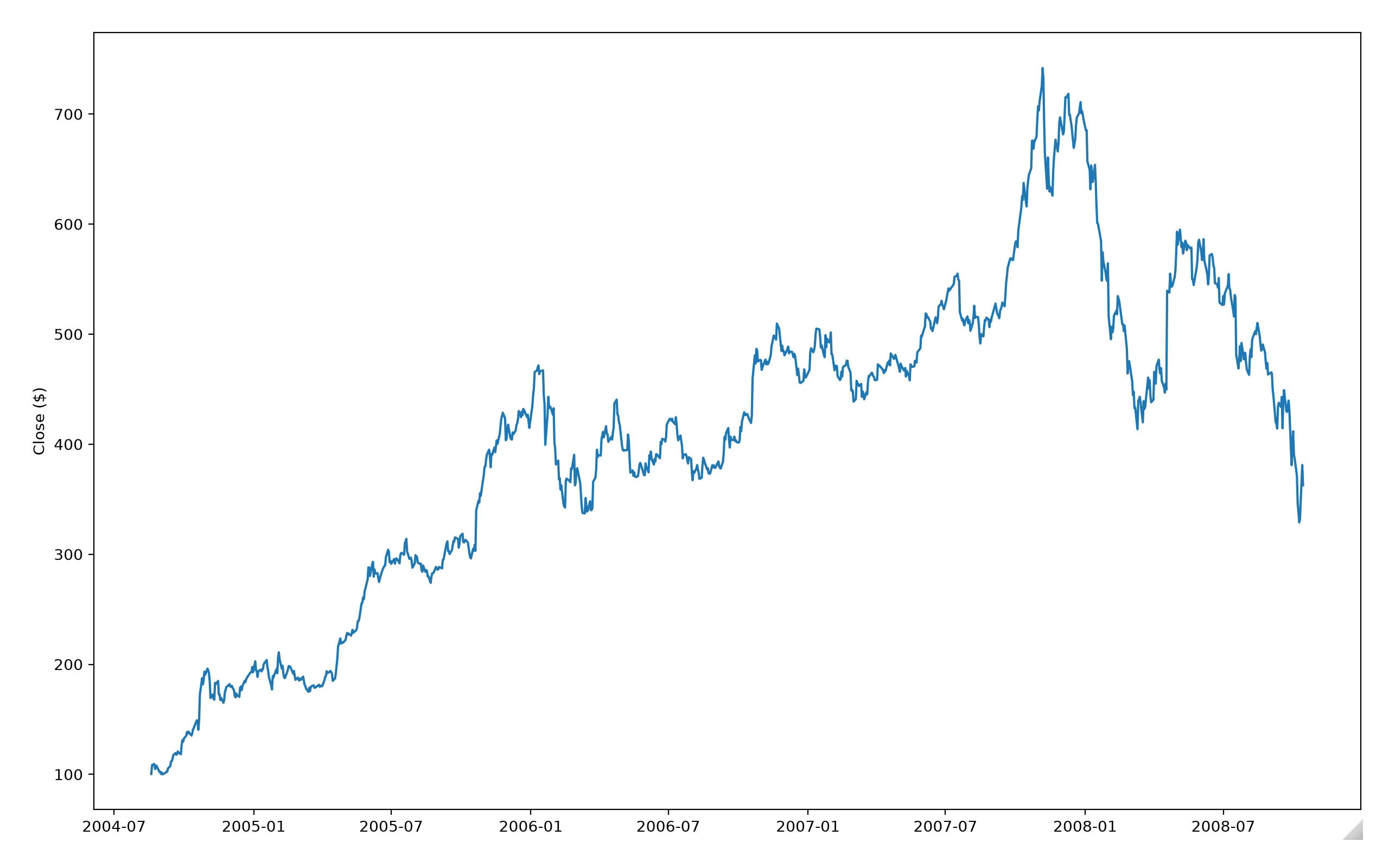

The figure renders with a toolbar (it fades in on hover): zoom-to-rectangle, pan, step back and forward through views, home, and download as PNG. Drag a box over the 2007-2008 runup and crash to see it:

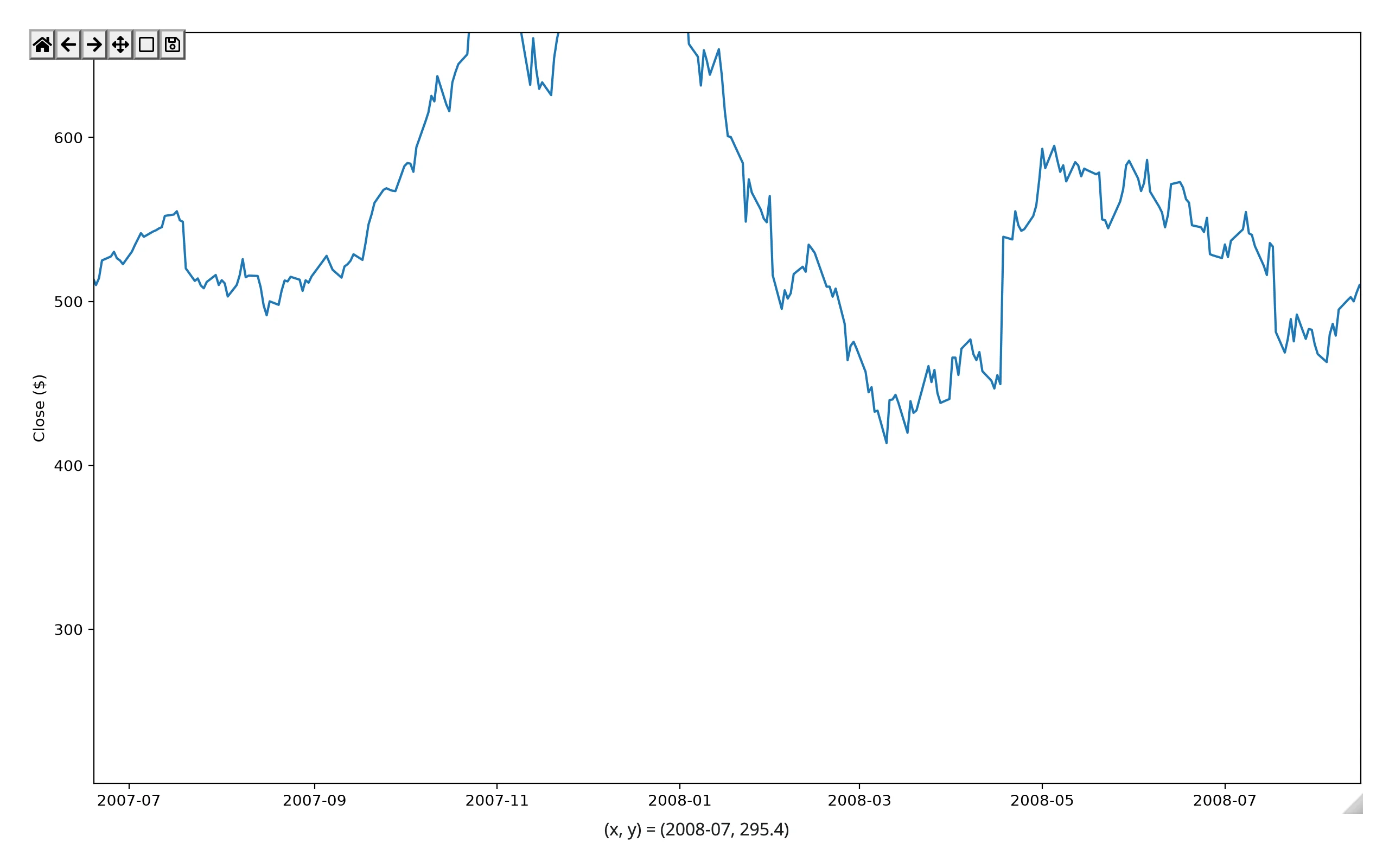
None of that – or anything below – is possible with a static @render.plot image.

What you can build

Anything built on matplotlib comes along for free. pandas’ .plot() accessor (and seaborn, statsmodels, scikit-learn displays, mplfinance) all return a Figure or Axes, so they render the same way (examples/02_pandas_plot.py):

examples/02_pandas_plot.py23 lines

import pandas as pd
from matplotlib.cbook import get_sample_data
from matplotlib.figure import Figure
from shiny.express import ui
from shinywidgets import render_matplotlib

ui.page_opts(fillable=True)

# Anything that hands matplotlib a Figure or Axes comes along for free:
# pandas' own .plot() accessor, seaborn, statsmodels, scikit-learn displays, ...
# Monthly adjusted close, 1990-2020ish, bundled with matplotlib as sample data
with get_sample_data("Stocks.csv") as f:
    stocks = pd.read_csv(f, comment="#", skipinitialspace=True, parse_dates=["Date"])
stocks = stocks.set_index("Date")[["AAPL", "MSFT", "GOOGL"]].dropna()


@render_matplotlib
def plot():
    fig = Figure(layout="constrained", figsize=(7, 4))
    ax = fig.subplots()
    stocks.plot(ax=ax, logy=True)
    ax.set_ylabel("Adjusted close ($, log scale)")
    return fig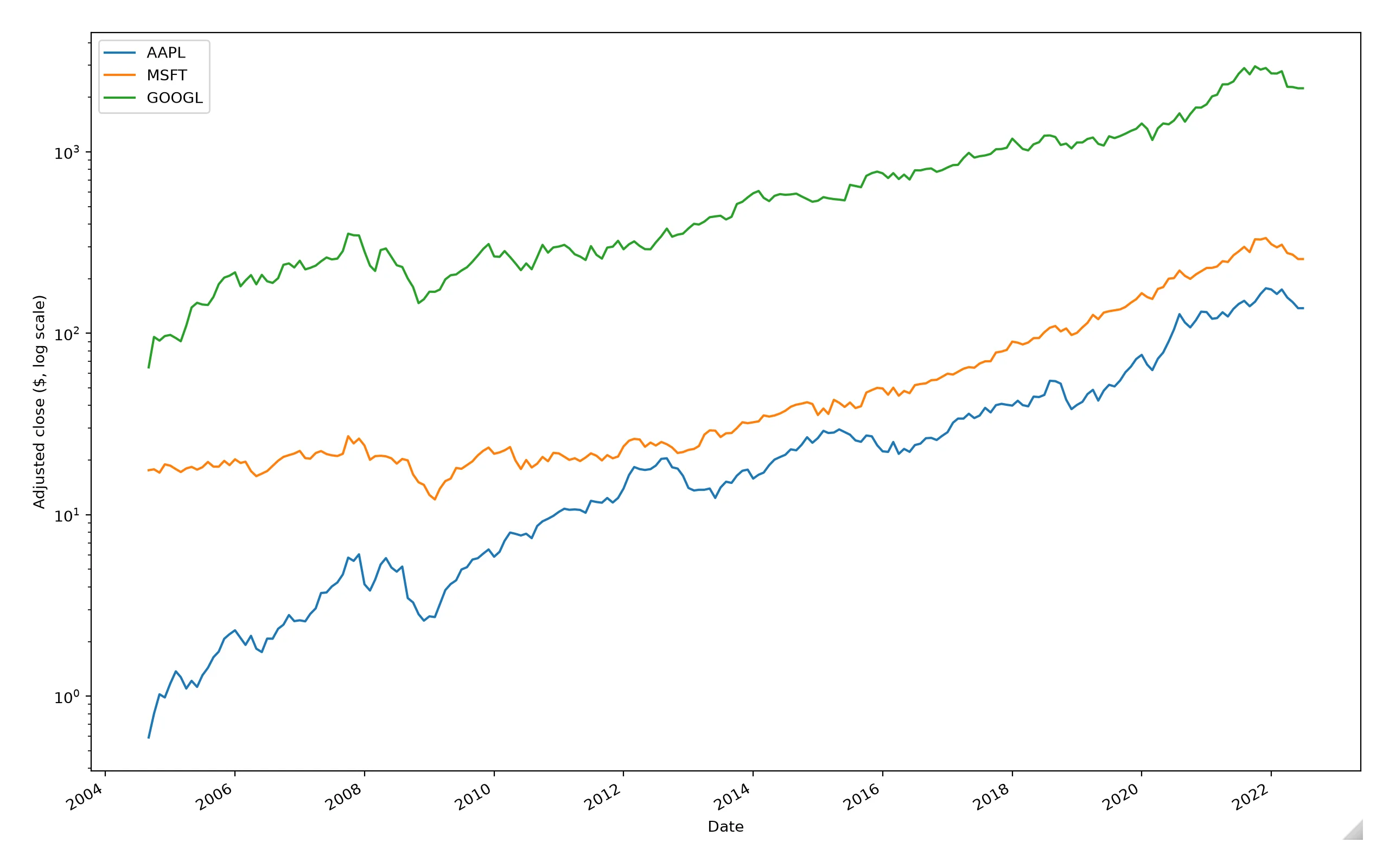

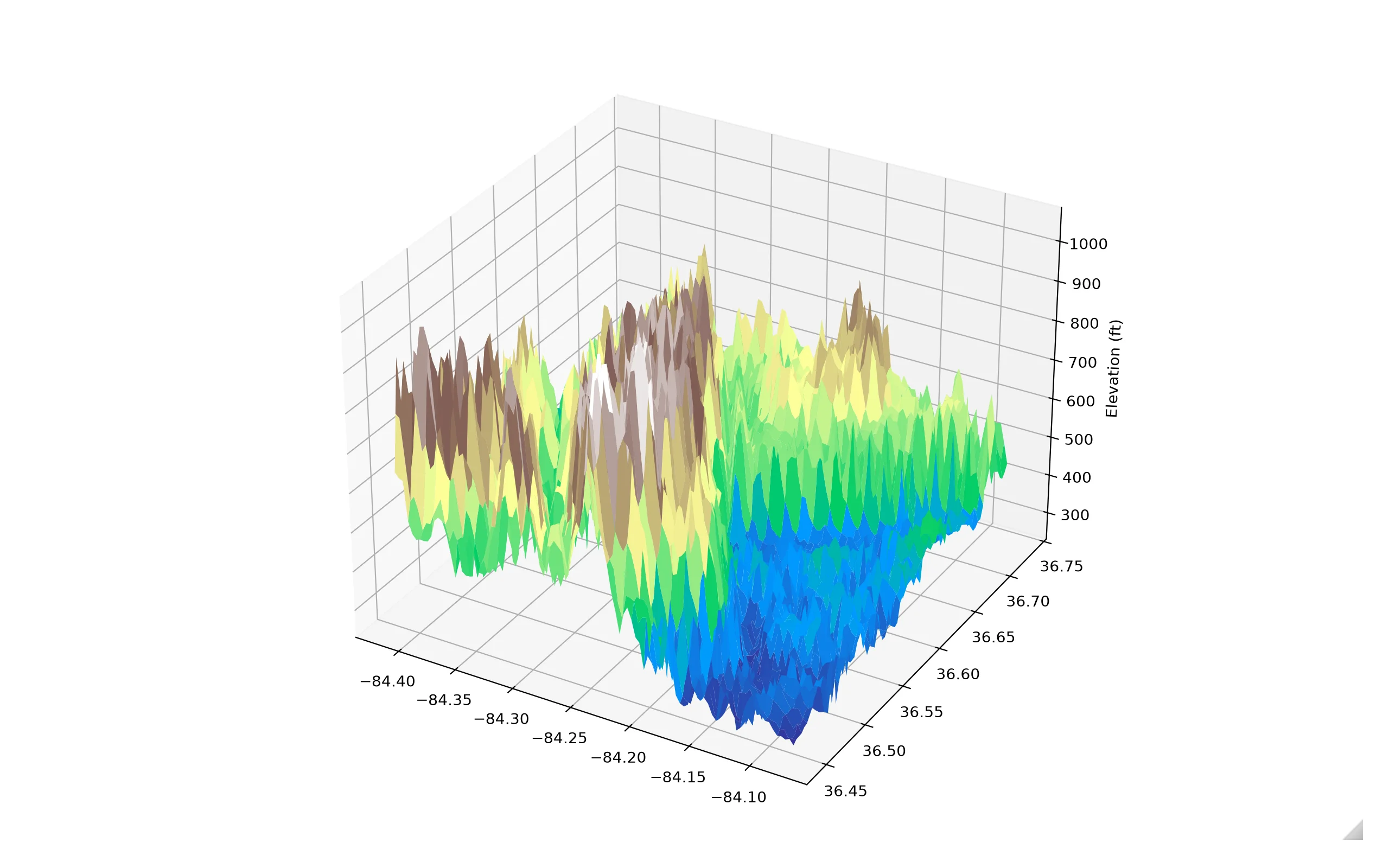
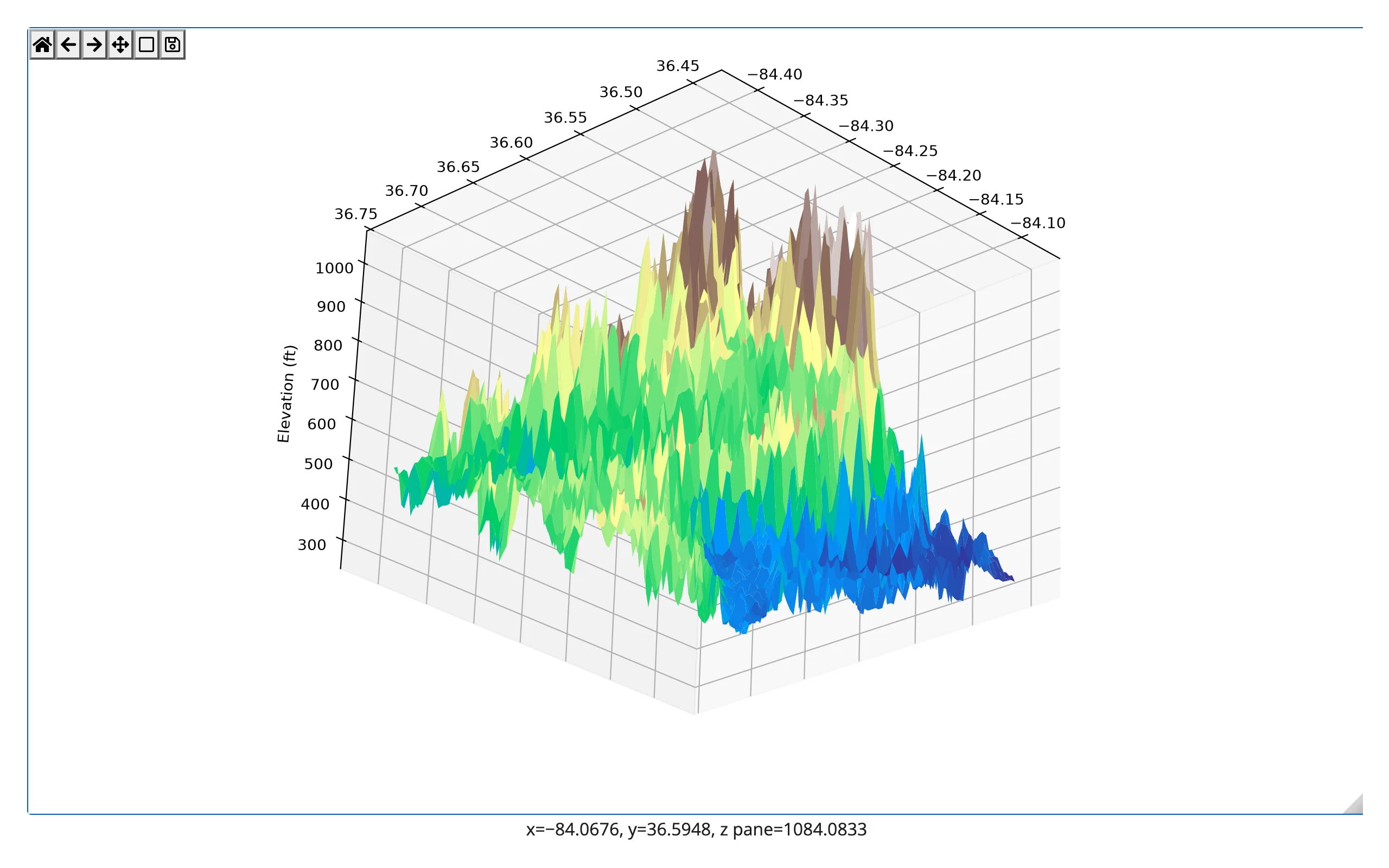
3D axes rotate by dragging, with no extra code – matplotlib’s own mplot3d toolkit handles the mouse events:

examples/03_rotate_3d.py23 lines

import numpy as np
from matplotlib.cbook import get_sample_data
from matplotlib.figure import Figure
from shiny.express import ui
from shinywidgets import render_matplotlib

ui.page_opts(fillable=True)

# A real elevation survey, bundled with matplotlib as sample data
dem = get_sample_data("jacksboro_fault_dem.npz")
z = dem["elevation"][::4, ::4]
x = np.linspace(dem["xmin"], dem["xmax"], z.shape[1])
y = np.linspace(dem["ymin"], dem["ymax"], z.shape[0])
X, Y = np.meshgrid(x, y)


@render_matplotlib
def plot():
    fig = Figure(layout="constrained")
    ax = fig.add_subplot(projection="3d")
    ax.plot_surface(X, Y, z, cmap="terrain")
    ax.set_zlabel("Elevation (ft)")
    return fig

Before drag	After drag

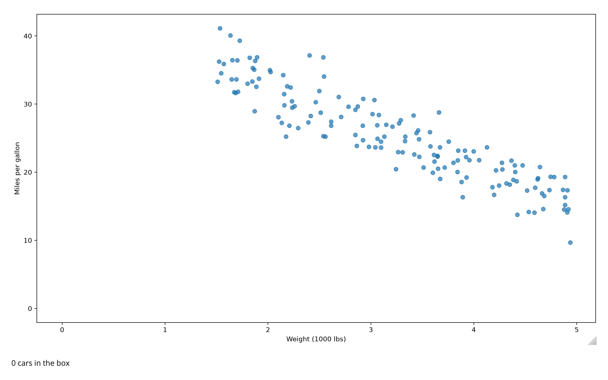
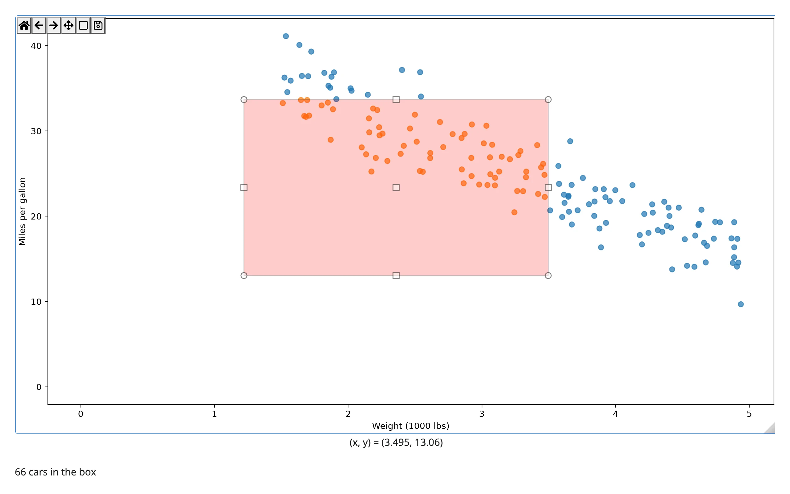
Matplotlib’s own interactive widgets (RectangleSelector, SpanSelector, sliders, buttons, …) work unmodified, because their callbacks are plain Python functions – which can set a reactive.value just like any other matplotlib event:

examples/04_rectangle_selector.py41 lines

import numpy as np
from matplotlib.figure import Figure
from matplotlib.widgets import RectangleSelector
from shiny import reactive
from shiny.express import render, ui
from shinywidgets import render_matplotlib

ui.page_opts(fillable=True)

# matplotlib's own widgets (selectors, sliders, buttons, ...) work unmodified:
# their callbacks are plain Python functions, so they can set reactive values.
rng = np.random.default_rng(2)
weight = rng.uniform(1.5, 5.0, 150)
mpg = 45 - 6 * weight + rng.normal(0, 2.5, 150)
n_selected = reactive.value(0)


@render_matplotlib
def plot():
    fig = Figure(layout="constrained")
    ax = fig.subplots()
    points = ax.scatter(weight, mpg, alpha=0.7)
    ax.set_xlabel("Weight (1000 lbs)")
    ax.set_ylabel("Miles per gallon")

    def on_select(press, release):
        x0, x1 = sorted([press.xdata, release.xdata])
        y0, y1 = sorted([press.ydata, release.ydata])
        mask = (weight >= x0) & (weight <= x1) & (mpg >= y0) & (mpg <= y1)
        points.set_facecolors(np.where(mask, "tab:orange", "tab:blue"))
        fig.canvas.draw_idle()
        n_selected.set(int(mask.sum()))

    # Keep a reference: matplotlib selectors stop working once garbage collected
    fig._selector = RectangleSelector(ax, on_select, interactive=True)
    return fig


@render.text
def summary():
    return f"{n_selected()} cars in the box"

Before	After dragging a box

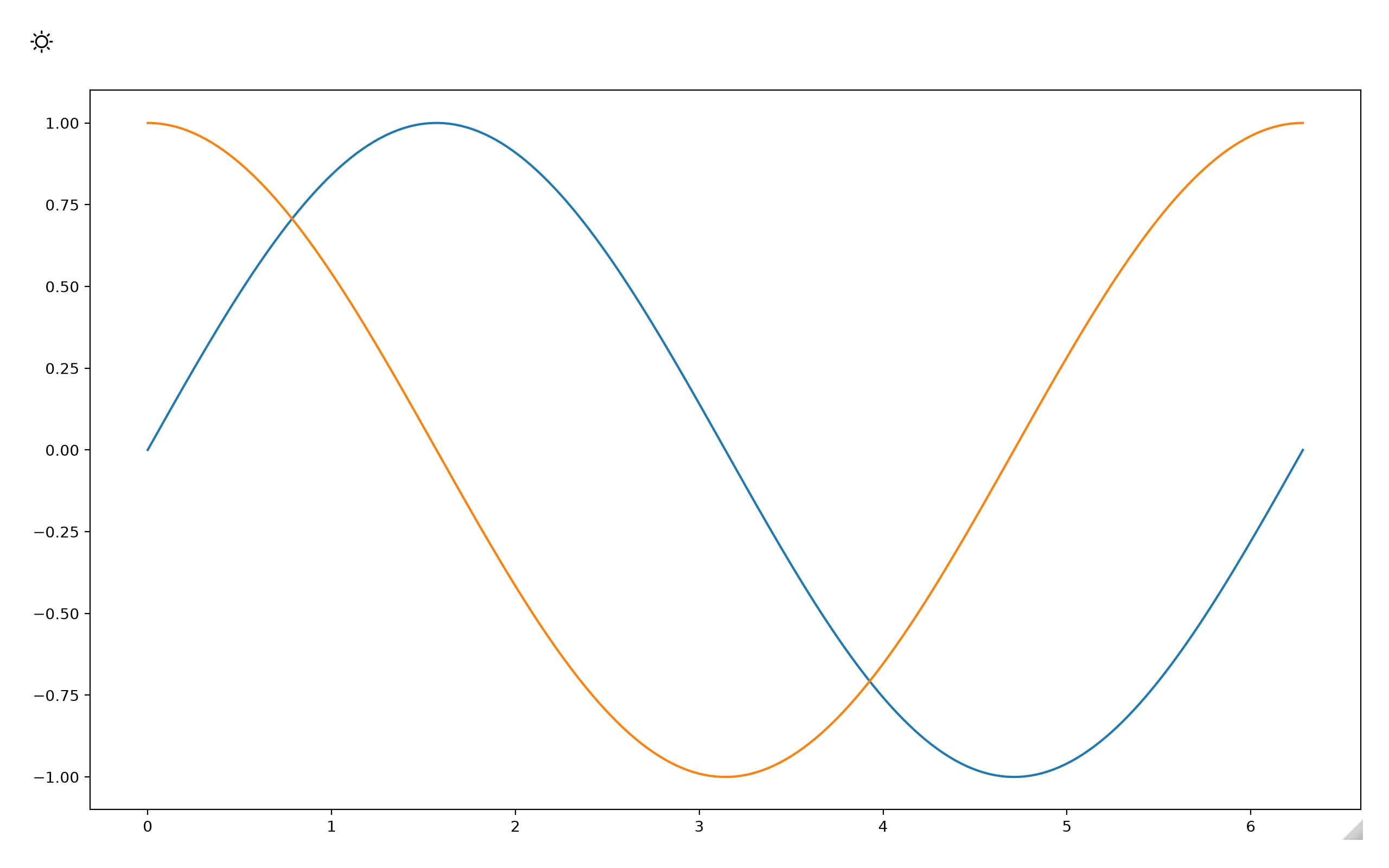
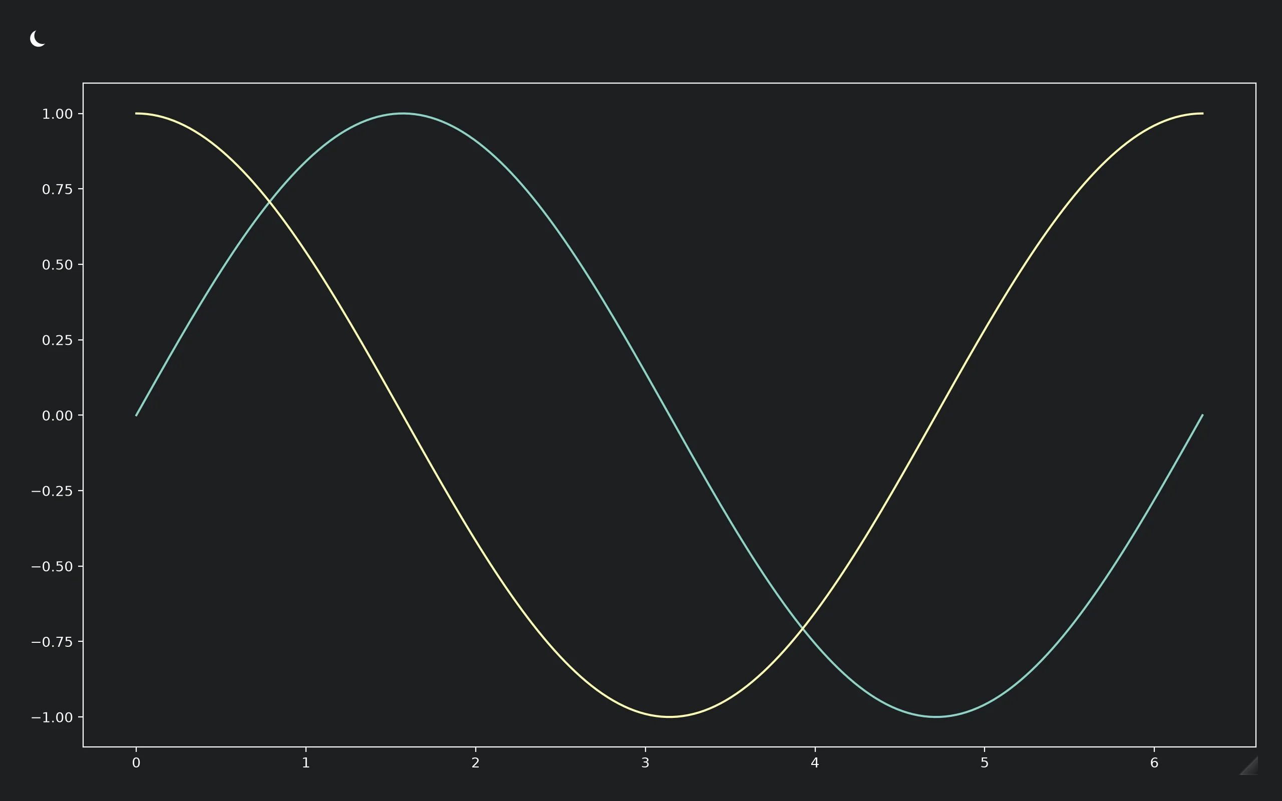
Figures can match bslib’s light/dark theme. Build the figure under plt.style.context() and make its background transparent so the card’s own color shows through:

examples/05_dark_mode.py25 lines

import matplotlib.pyplot as plt
import numpy as np
from matplotlib.figure import Figure
from shiny.express import input, ui
from shinywidgets import render_matplotlib

ui.page_opts(fillable=True)
ui.input_dark_mode(id="mode")

t = np.linspace(0, 2 * np.pi, 200)


@render_matplotlib
def plot():
    style = "dark_background" if input.mode() == "dark" else "default"
    with plt.style.context(style):
        fig = Figure(layout="constrained")
        ax = fig.subplots()
        ax.plot(t, np.sin(t))
        ax.plot(t, np.cos(t))
    # Transparent background so the card's own color shows through instead of
    # matplotlib's opaque white/black
    fig.patch.set_alpha(0)
    ax.patch.set_alpha(0)
    return fig

Light	Dark

Re-rendering on a mode switch resets zoom, since it rebuilds the figure; see Updating the widget from Python to change styling without losing the user’s view.

Reacting to user interaction

The output gains methods that read what the user does to the figure, much like input.my_slider() reads an input. Call them in a reactive context (a @render.* function, @reactive.calc, or @reactive.effect), which re-runs whenever the value changes.

Accessor reference

Accessor	Returns	Before any interaction	Across re-render	Default rate policy
`clicked()`	`matplotlib.backend_bases.MouseEvent`	`None`	kept (payload describes the previous render’s figure)	not rate-limited
`picked()`	`matplotlib.backend_bases.PickEvent`	`None`	kept (payload describes the previous render’s figure)	not rate-limited
`limits(ax=0)`	`((x0, x1), (y0, y1))` for axes `ax`	seeded value (the figure’s rendered limits)	re-seeded from the new figure	debounced, 250 ms

clicked() and picked() attach the moment the figure renders and record a press whether or not anything has read them yet – there’s no warm-up to write. limits() behaves differently on re-render: because it’s the figure’s own view state, not something the user did, it re-seeds from the new figure’s limits rather than carrying over the old zoom (verified by re-rendering a zoomed figure and reading limits() immediately after – it reports the new figure’s full extent, not the old window). clicked() and picked(), by contrast, keep reporting the last press on the previous figure until the user interacts with the new one.

`clicked()`: inspect a point

examples/06_accessor_clicked.py24 lines

import numpy as np
from matplotlib.figure import Figure
from shiny import req
from shiny.express import render, ui
from shinywidgets import render_matplotlib

ui.page_opts(fillable=True)

t = np.linspace(0, 10, 300)
signal = np.sin(t) + 0.15 * np.random.default_rng(0).standard_normal(300)


@render_matplotlib
def plot():
    fig = Figure(layout="constrained")
    ax = fig.subplots()
    ax.plot(t, signal, lw=1)
    return fig


@render.code
def reading():
    ev = req(plot.clicked())
    return f"x={ev.xdata:.2f}  y={ev.ydata:.2f}"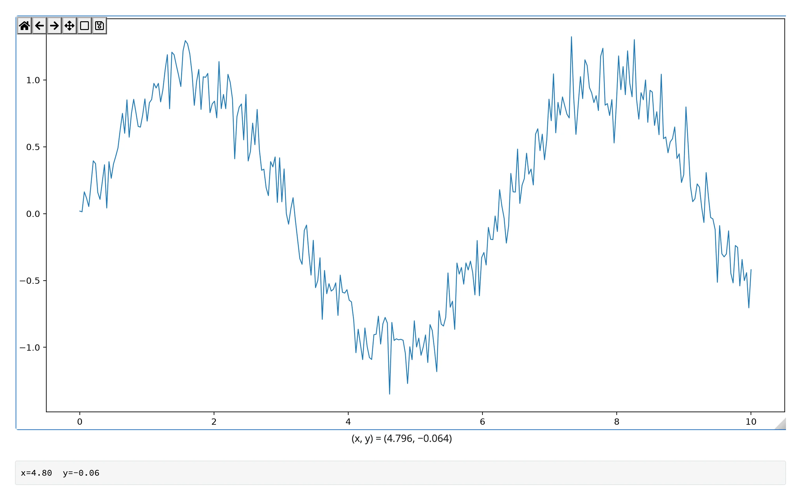

.xdata/.ydata are in the data coordinates of the axes under the press (.inaxes). Every press fires – clicked() doesn’t deduplicate, so a double-click arrives as three presses. A press that starts a toolbar pan/zoom drag, or lands outside any axes, doesn’t count: if you’ve just used the zoom or pan tool, click it again to turn it off before clicking a point, or the press is ignored (verified – see Gotchas). clicked() attaches the moment the figure renders, so a press is recorded even if nothing has read it yet, and it keeps its value across a re-render until the user clicks the new figure – the event then describes the previous render’s figure, so prefer an ID-keyed lookup over a positional index if your data can change shape between renders.

`picked()`: identify an artist

Only artists created with picker= are pickable (e.g. ax.scatter(..., picker=5), where 5 is the hit-test tolerance in points):

examples/07_accessor_picked.py28 lines

import numpy as np
from matplotlib.figure import Figure
from shiny import req
from shiny.express import render, ui
from shinywidgets import render_matplotlib

ui.page_opts(fillable=True)

cities = ["Austin", "Boise", "Chicago", "Denver", "Eugene", "Fargo"]
pop = np.array([980, 235, 2700, 715, 175, 125])
growth = np.array([2.8, 3.1, 0.4, 2.2, 1.6, 0.9])


@render_matplotlib
def plot():
    fig = Figure(layout="constrained")
    ax = fig.subplots()
    ax.scatter(pop, growth, s=80, picker=5)
    ax.set_xlabel("Population (thousands)")
    ax.set_ylabel("Growth rate (%)")
    return fig


@render.code
def picked():
    ev = req(plot.picked())
    i = ev.ind[0]
    return f"{cities[i]}: {pop[i]}k people, {growth[i]}% growth"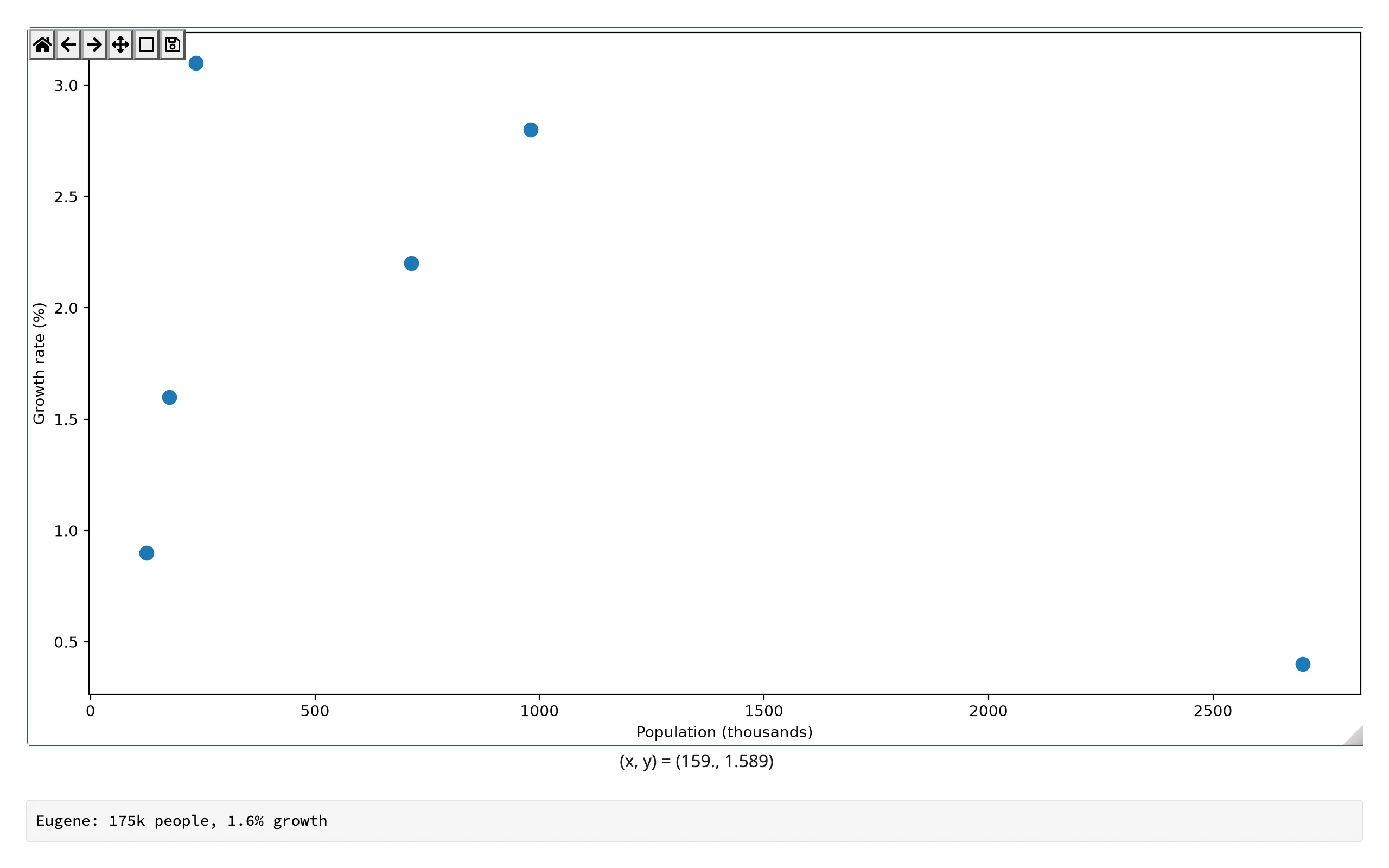

.ind is a tuple of indices into the picked artist’s data arrays – for an exact line, usually one index; for a dense scatter, every point under the cursor. Like clicked(), picked() attaches at render and keeps its value across a re-render until the user picks something on the new figure.

`limits(ax=0)`: zoom is a query

examples/08_accessor_limits.py23 lines

import numpy as np
from matplotlib.figure import Figure
from shiny.express import render, ui
from shinywidgets import render_matplotlib

ui.page_opts(fillable=True)

t = np.linspace(0, 100, 5000)
y = np.sin(t) + 0.05 * t


@render_matplotlib
def plot():
    fig = Figure(layout="constrained")
    ax = fig.subplots()
    ax.plot(t, y, lw=0.8)
    return fig


@render.code
def window():
    (x0, x1), (y0, y1) = plot.limits()
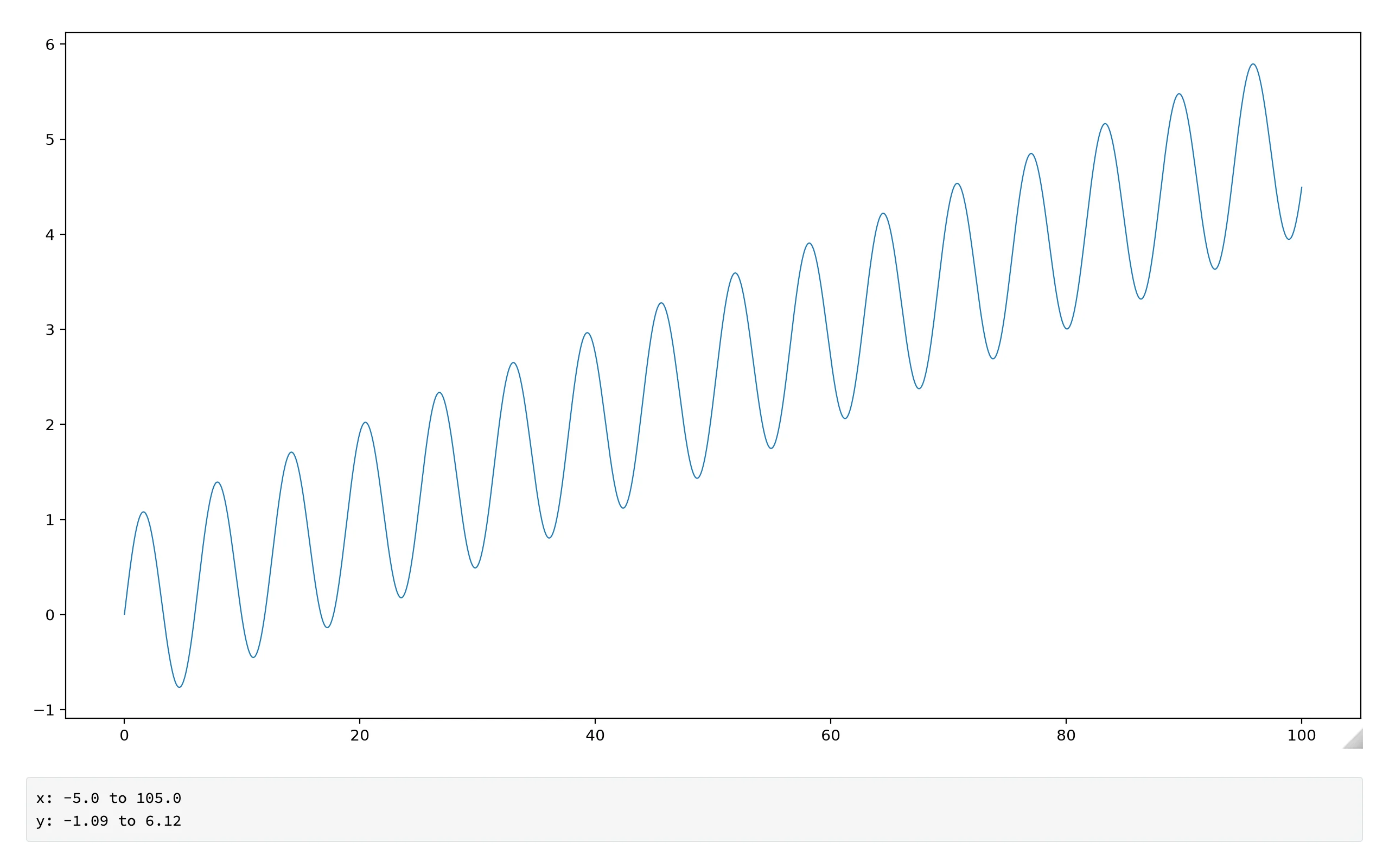
    return f"x: {x0:.1f} to {x1:.1f}\ny: {y0:.2f} to {y1:.2f}"

Before zoom	After zoom

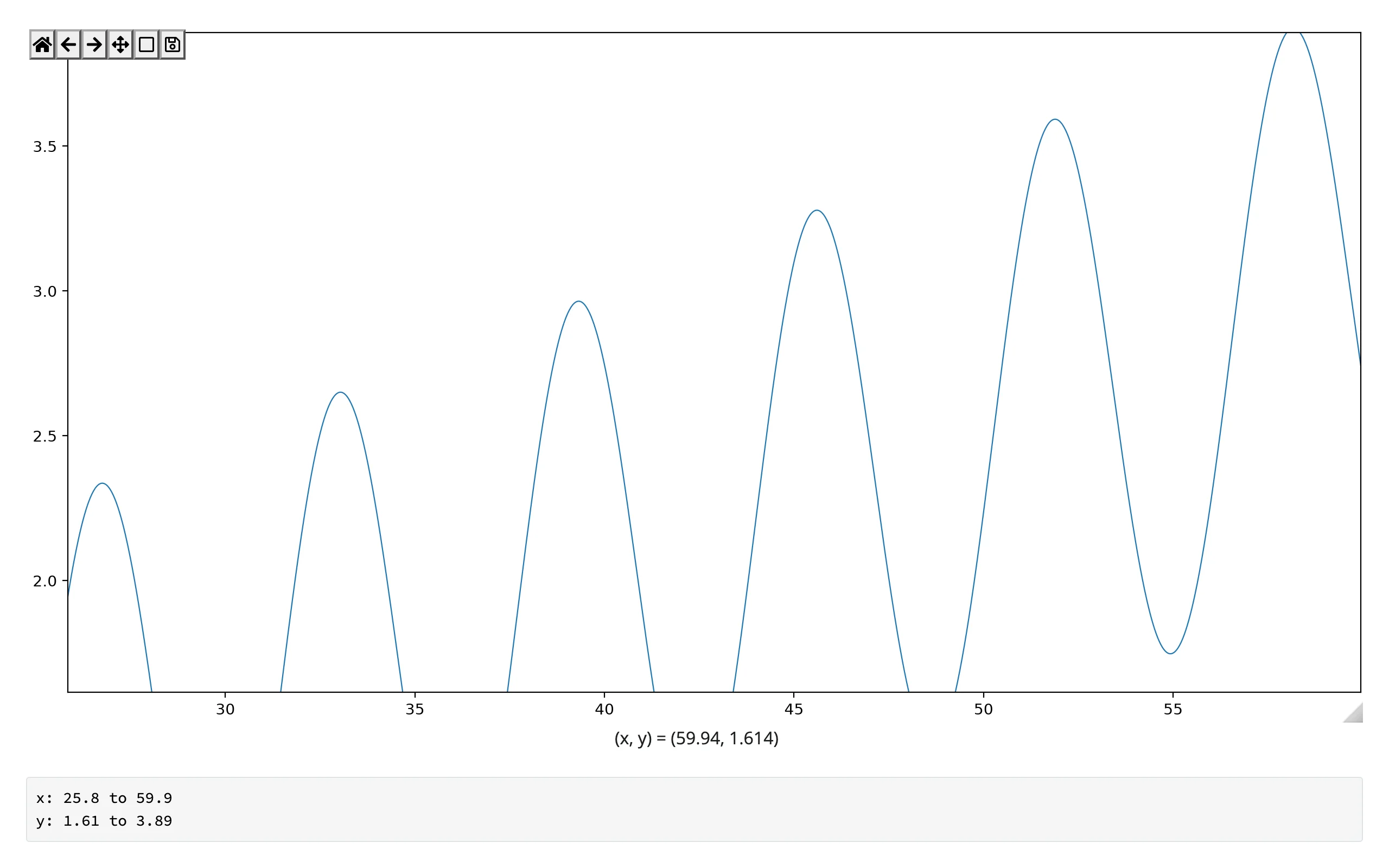limits() is seeded from the figure’s rendered limits, then updates after every zoom or pan step – including ones made from Python (e.g. ax.set_xlim(...) in an effect). ax indexes .widget.figure.axes, so limits(ax=1) reads a second subplot; an out-of-range index raises IndexError naming how many axes the figure has. It can’t be read inside the plot’s own render function (which builds a new figure every run) – read it in another output or an effect instead. Unlike clicked()/picked(), a re-render re-seeds limits() from the new figure’s own limits rather than carrying over the old zoom window – it describes the figure’s current view, not a user action, so there’s nothing to carry over.

Reading an accessor on demand

Because every accessor is live from the moment the figure renders, it’s safe to read one anywhere – a button handler, a download handler, a @reactive.event – not just from an output that’s always on screen. Here, a “Save current view” button reads plot.limits() on click and appends it to a running list, with no warm-up @reactive.effect needed to make the first read work:

examples/16_read_on_demand.py35 lines

import numpy as np
from matplotlib.figure import Figure
from shiny import reactive
from shiny.express import input, render, ui
from shinywidgets import render_matplotlib

ui.page_opts(fillable=True)
ui.input_action_button("save", "Save current view")

t = np.linspace(0, 50, 4000)
y = np.sin(t) + 0.3 * np.sin(5 * t) + 0.02 * t**1.2
bookmarks = reactive.value([])


@render_matplotlib
def plot():
    fig = Figure(layout="constrained")
    ax = fig.subplots()
    ax.plot(t, y, lw=0.8)
    return fig


@reactive.effect
@reactive.event(input.save)
def _save_view():
    (x0, x1), _ = plot.limits()
    bookmarks.set([*bookmarks(), f"{x0:.1f} to {x1:.1f}"])


@render.code
def saved():
    views = bookmarks()
    if not views:
        return "No views saved yet -- zoom in, then click Save."
    return "\n".join(f"{i + 1}. {v}" for i, v in enumerate(views))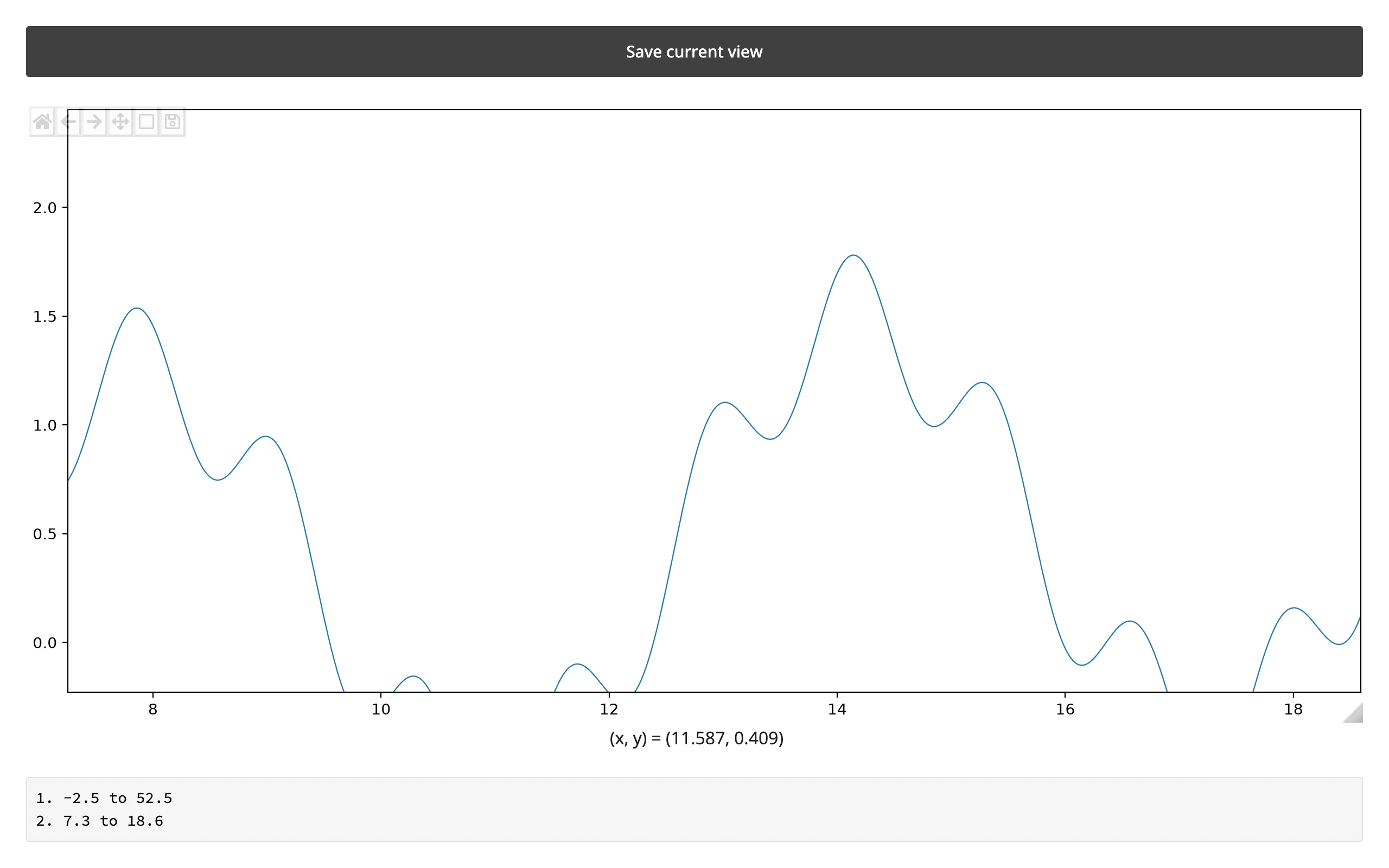

Verified: clicking Save before any zoom records the figure’s full extent (limits() is already seeded, not None); zooming in and clicking Save again appends the new window. Each click reads plot.limits() fresh – it isn’t a dependency of saved(), so saving a view doesn’t by itself re-run anything except the effect that records it.

Beyond the accessors: `.read()` and reactive_read

ipympl’s Canvas has no synced trait worth reading with plot.read(...) (which falls through to reactive_read() for names that aren’t accessors) – its traits are chrome (header_visible, toolbar_position, …) or private. For anything the three accessors don’t cover (hover, key presses, scroll, custom selectors), connect matplotlib’s own callbacks and set a reactive.value from them, same as the RectangleSelector example above:

examples/09_beyond_accessors_hover.py31 lines

import numpy as np
from matplotlib.figure import Figure
from shiny import reactive
from shiny.express import render, ui
from shinywidgets import render_matplotlib

ui.page_opts(fillable=True)

t = np.linspace(0, 10, 300)
y = np.sin(t)
hover = reactive.value("move the mouse over the plot")


@render_matplotlib
def plot():
    fig = Figure(layout="constrained")
    ax = fig.subplots()
    ax.plot(t, y)

    def on_move(event):
        if event.inaxes is None:
            return
        hover.set(f"x={event.xdata:.2f}  y={event.ydata:.2f}")

    fig.canvas.mpl_connect("motion_notify_event", on_move)
    return fig


@render.code
def coords():
    return hover()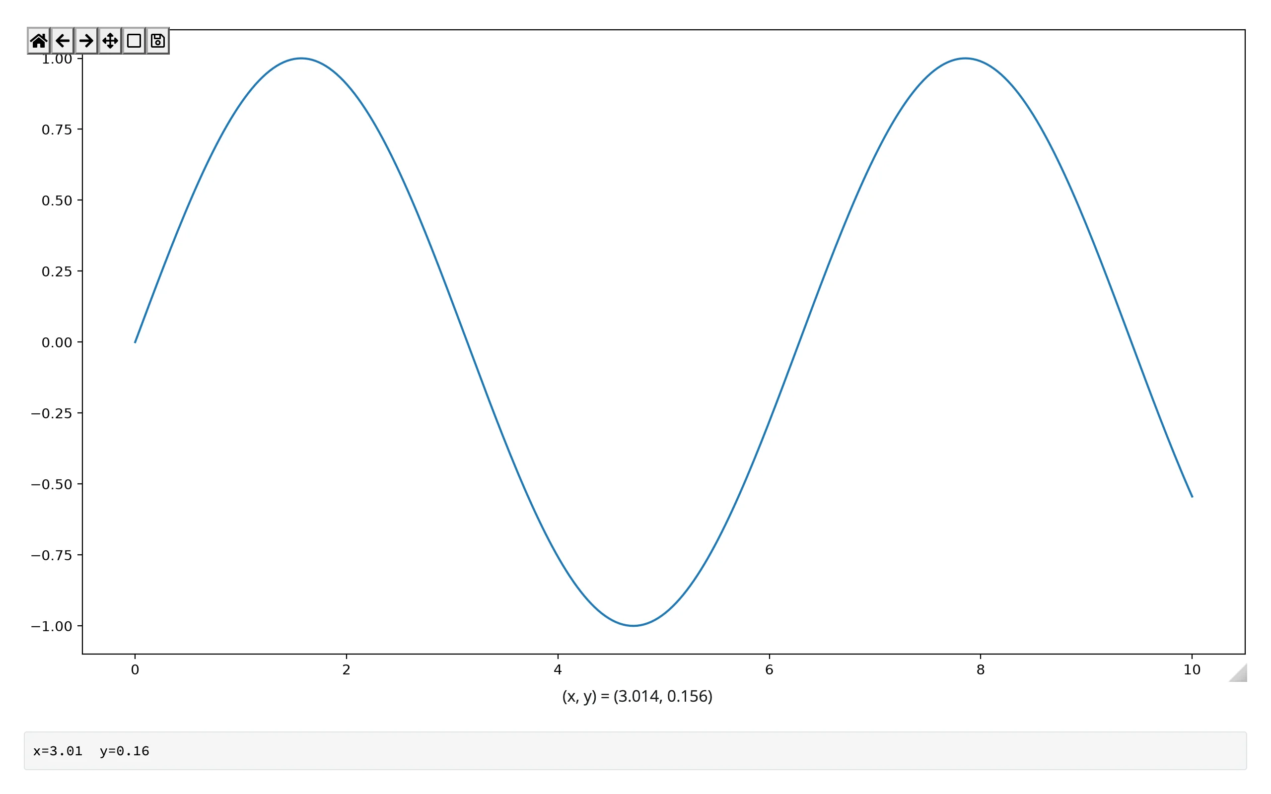

Other hooks worth knowing: "key_press_event" (the figure needs focus – click it first), "scroll_event" (disabled by default; set canvas.capture_scroll = True), and ax.callbacks.connect("ylim_changed", ...) if you need the y-limits without the x (limits() returns both together).

Rate limiting

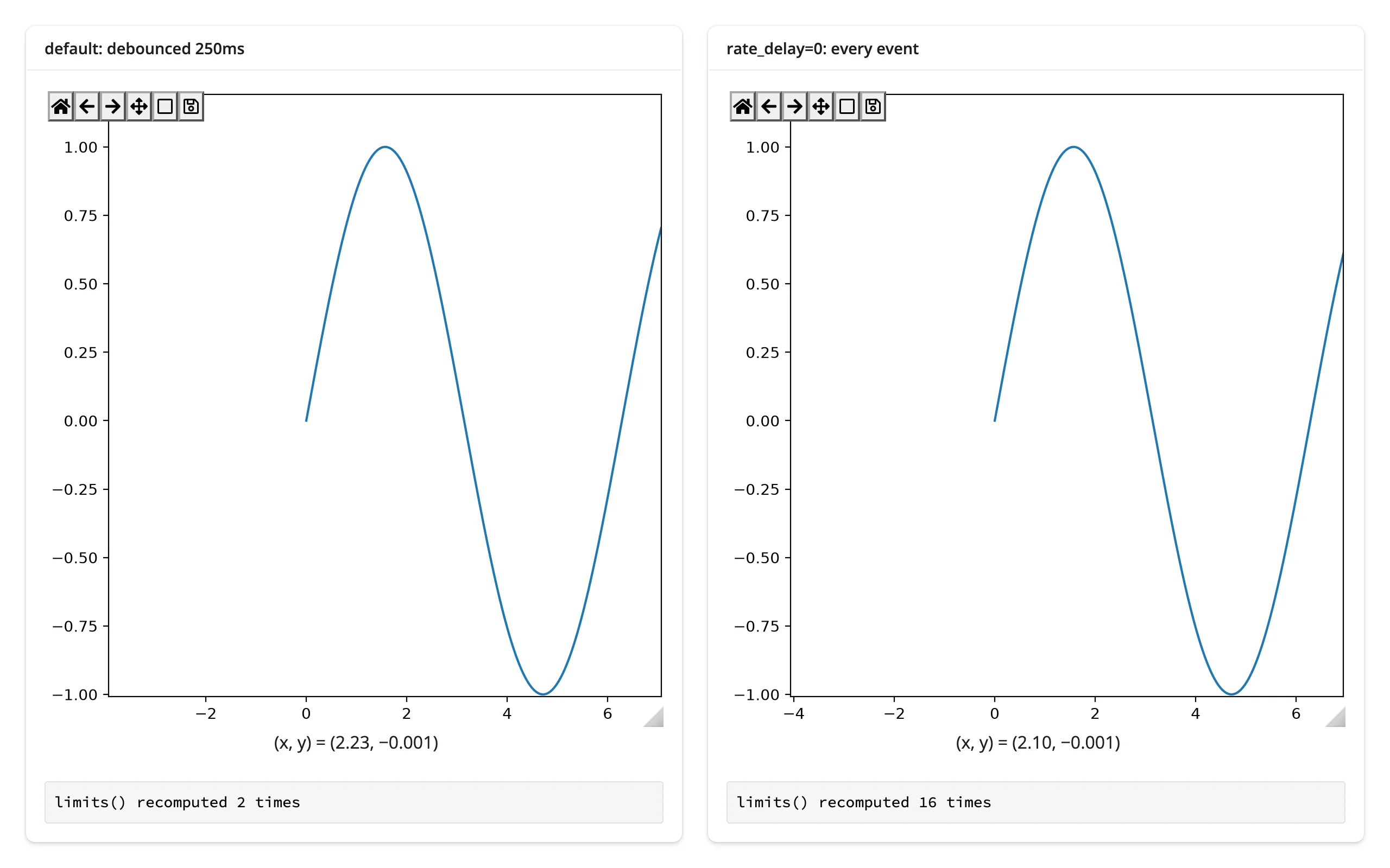
limits() is debounced 250 ms by default – a zoom-to-rectangle drag fires about a dozen xlim_changed/ ylim_changed events, and only the settled value after the pause reaches Python. Pass rate_delay=0 to react to every event instead (e.g. to drive a second plot smoothly while panning), or rate_policy="throttle" to get evenly-spaced updates during a long drag rather than waiting for it to stop:

examples/10_rate_limiting.py47 lines

import numpy as np
from matplotlib.figure import Figure
from shiny.express import render, ui
from shinywidgets import as_widget, render_matplotlib

ui.page_opts(fillable=True)

t = np.linspace(0, 10, 2000)
y = np.sin(t)
counts = {"default": 0, "fast": 0}


def make_plot():
    fig = Figure(layout="constrained", figsize=(4, 3))
    ax = fig.subplots()
    ax.plot(t, y)
    canvas = as_widget(fig)
    canvas.toolbar_visible = "visible"  # skip the hover-to-reveal fade
    return canvas


with ui.layout_columns():
    with ui.card():
        ui.card_header("default: debounced 250ms")

        @render_matplotlib
        def default_out():
            return make_plot()

        @render.code
        def default_count():
            default_out.limits()
            counts["default"] += 1
            return f"limits() recomputed {counts['default']} times"

    with ui.card():
        ui.card_header("rate_delay=0: every event")

        @render_matplotlib(rate_delay=0)
        def fast_out():
            return make_plot()

        @render.code
        def fast_count():
            fast_out.limits()
            counts["fast"] += 1
            return f"limits() recomputed {counts['fast']} times"

Panning the same distance on both plots (verified with a scripted drag): the debounced plot recomputed twice (the initial seed, then the settled value), the rate_delay=0 plot recomputed 16 times.

Updating the widget from Python

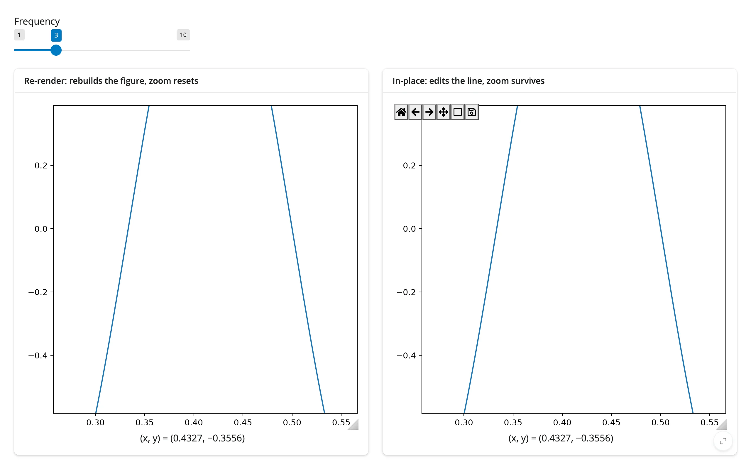
The decorated function gains a read-only .widget attribute – the rendered Canvas – once it has rendered. Editing its figure’s artists and calling .widget.draw_idle() updates the picture without re-rendering the widget: the user’s zoom, pan position, and any pending selection survive, and no new comm handshake or JS bundle has to ship to the browser. Re-rendering (returning a new figure from the decorated function) is simpler, but rebuilds the Canvas from scratch, so the view resets.

Use in-place updates when the figure’s zoom/pan state matters to the user (dashboards, exploratory tools); re-render when the shape of the plot itself changes (different number of subplots, totally different data) or when simplicity matters more than preserving view state.

examples/11_inplace_vs_rerender.py50 lines

import numpy as np
from matplotlib.figure import Figure
from shiny import reactive
from shiny.express import input, ui
from shinywidgets import render_matplotlib

ui.page_opts(fillable=True)
ui.input_slider("freq", "Frequency", 1, 10, 3)

x = np.linspace(0, 1, 400)


def base_plot():
    fig = Figure(layout="constrained", figsize=(4, 3))
    ax = fig.subplots()
    ax.plot(x, np.sin(2 * np.pi * 3 * x))
    ax.set_ylim(-1.1, 1.1)
    return fig


with ui.layout_columns():
    with ui.card(full_screen=True):
        ui.card_header("Re-render: rebuilds the figure, zoom resets")

        @render_matplotlib
        def rerendered():
            fig = Figure(layout="constrained", figsize=(4, 3))
            ax = fig.subplots()
            ax.plot(x, np.sin(2 * np.pi * input.freq() * x))
            ax.set_ylim(-1.1, 1.1)
            return fig

    with ui.card(full_screen=True):
        ui.card_header("In-place: edits the line, zoom survives")

        @render_matplotlib
        def inplace():
            # Doesn't depend on input.freq(): built once, edited afterward
            return base_plot()


@reactive.effect
def _():
    with reactive.isolate():
        canvas = inplace.widget
    if canvas is None:
        return
    line = canvas.figure.axes[0].lines[0]
    line.set_ydata(np.sin(2 * np.pi * input.freq() * x))
    canvas.draw_idle()

Both panels zoomed to the same region, then the frequency slider moved from 3 to 8:

Both zoomed in	After moving the slider

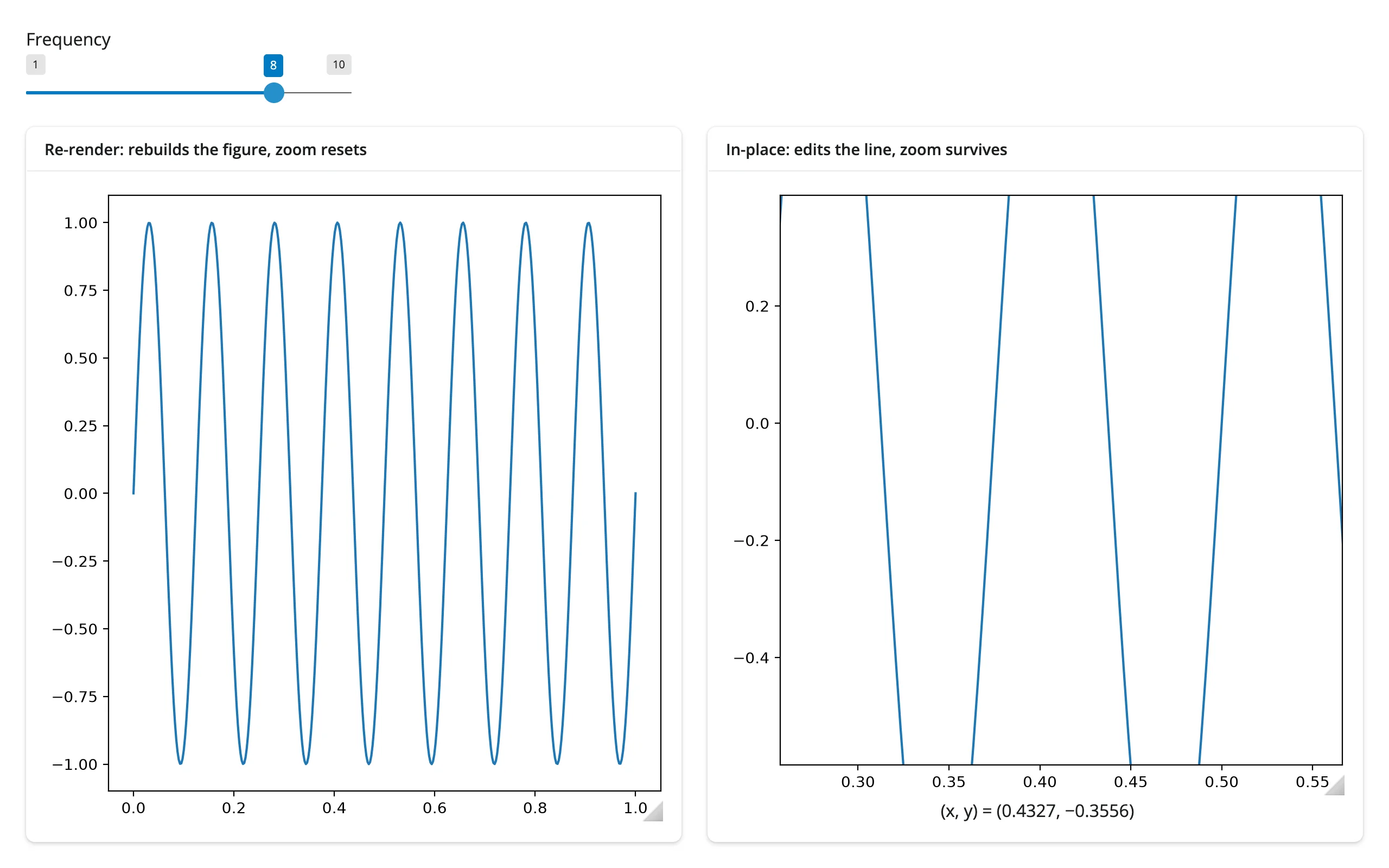The left panel snaps back to the full x-axis range (a fresh Figure, fresh axes limits); the right panel keeps the exact zoomed window while its line restyles underneath.

reactive.isolate() around the .widget read keeps the effect from depending on every render of inplace (it would otherwise re-run whenever the widget identity changed, pointlessly). Read inputs normally outside the isolate block so the effect still re-runs when they change. The same pattern drives animation and streaming: a reactive.effect that calls reactive.invalidate_later(dt) and edits the figure on each tick delivers updates to the browser immediately on current Shiny (>= 1.9, verified with four ticks over 2.4s with no client interaction) – call relim()/autoscale_view() first if the data range changes.

Coordinating multiple views

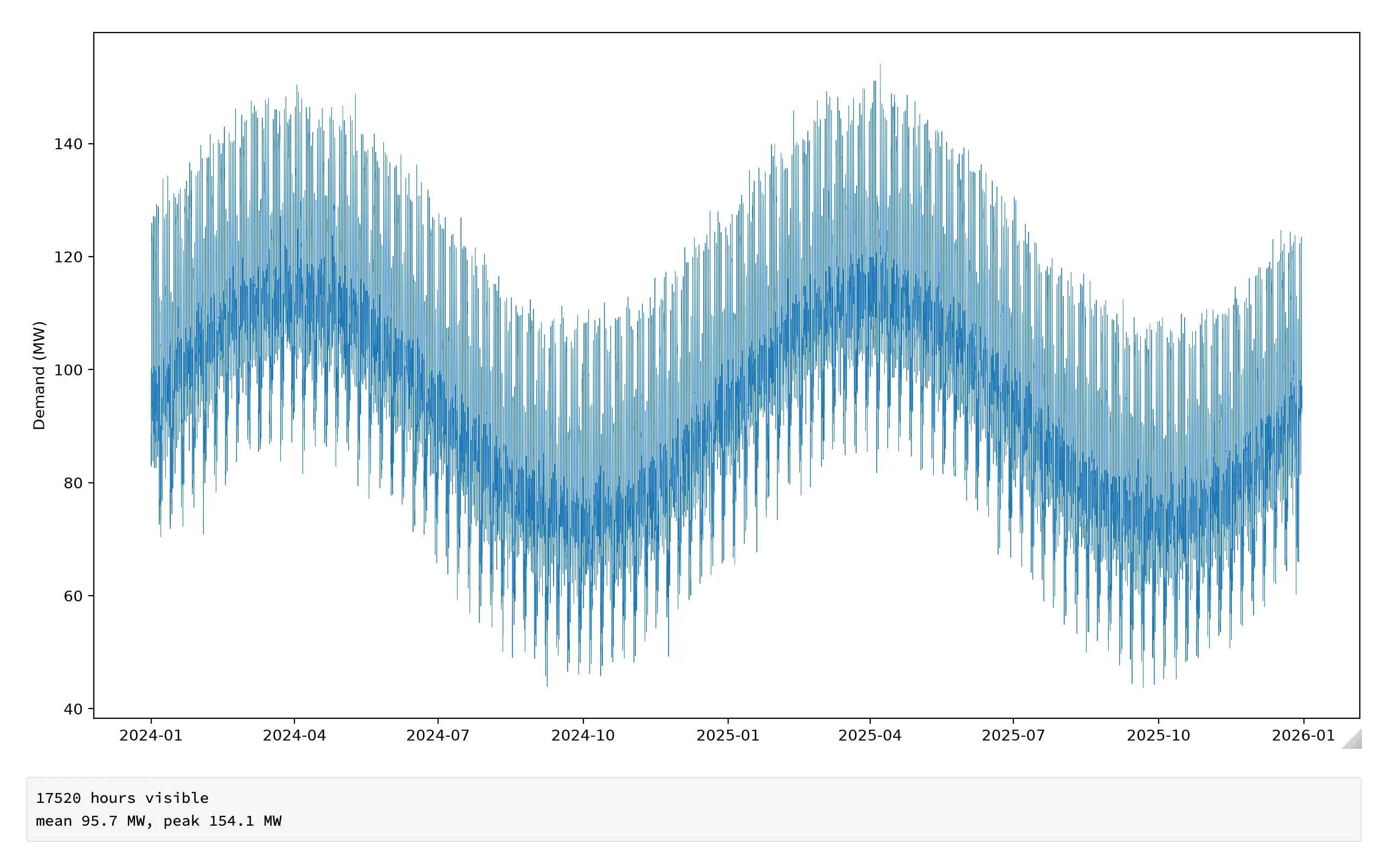
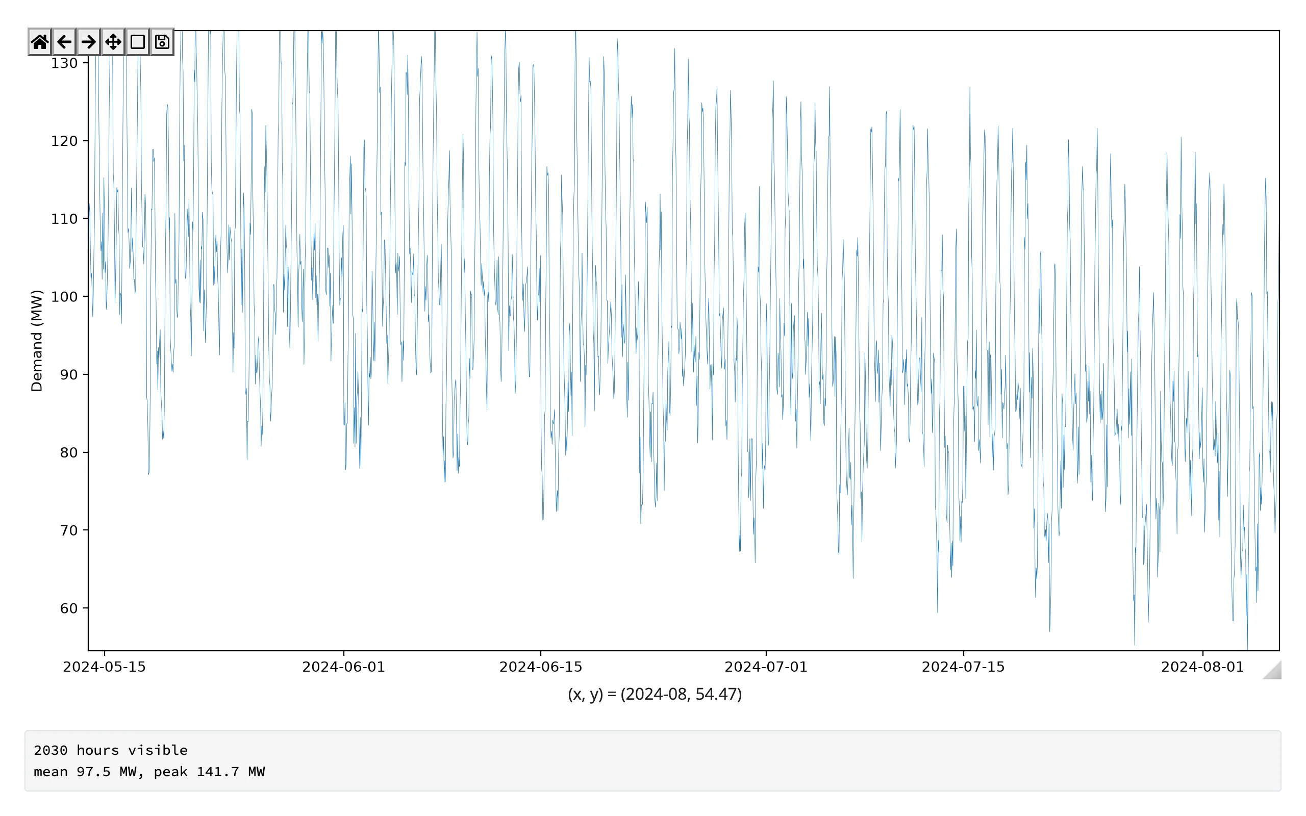
Zoom drives a summary panel

examples/12_coordinate_zoom_summary.py46 lines

import numpy as np
import pandas as pd
from matplotlib.dates import num2date
from matplotlib.figure import Figure
from shiny.express import render, ui
from shinywidgets import render_matplotlib

ui.page_opts(fillable=True)

# Two years of hourly demand with a seasonal cycle, a daily double-peak, and
# quiet weekends -- the kind of series where "what happened in this window?"
# only makes sense once you've zoomed into it.
hours = pd.date_range("2024-01-01", periods=24 * 365 * 2, freq="h")
hour_of_day = hours.hour.to_numpy()
rng = np.random.default_rng(3)
demand = (
    100
    + 20 * np.sin(2 * np.pi * hours.dayofyear.to_numpy() / 365)
    + 15 * np.sin(2 * np.pi * (hour_of_day - 6) / 24)
    + 10 * np.sin(4 * np.pi * (hour_of_day - 8) / 24)
    - 15 * (hours.dayofweek.to_numpy() >= 5)
    + rng.normal(0, 3, len(hours))
)


@render_matplotlib
def plot():
    fig = Figure(layout="constrained")
    ax = fig.subplots()
    ax.plot(hours, demand, lw=0.3)
    ax.set_ylabel("Demand (MW)")
    return fig


@render.code
def summary():
    (x0, x1), _ = plot.limits()
    start, end = num2date(x0).replace(tzinfo=None), num2date(x1).replace(tzinfo=None)
    mask = (hours >= pd.Timestamp(start)) & (hours <= pd.Timestamp(end))
    visible = demand[mask]
    if visible.size == 0:
        return "Zoom in to see a summary of the visible window"
    return (
        f"{visible.size} hours visible\n"
        f"mean {visible.mean():.1f} MW, peak {visible.max():.1f} MW"
    )

Full range	Zoomed to 6 weeks

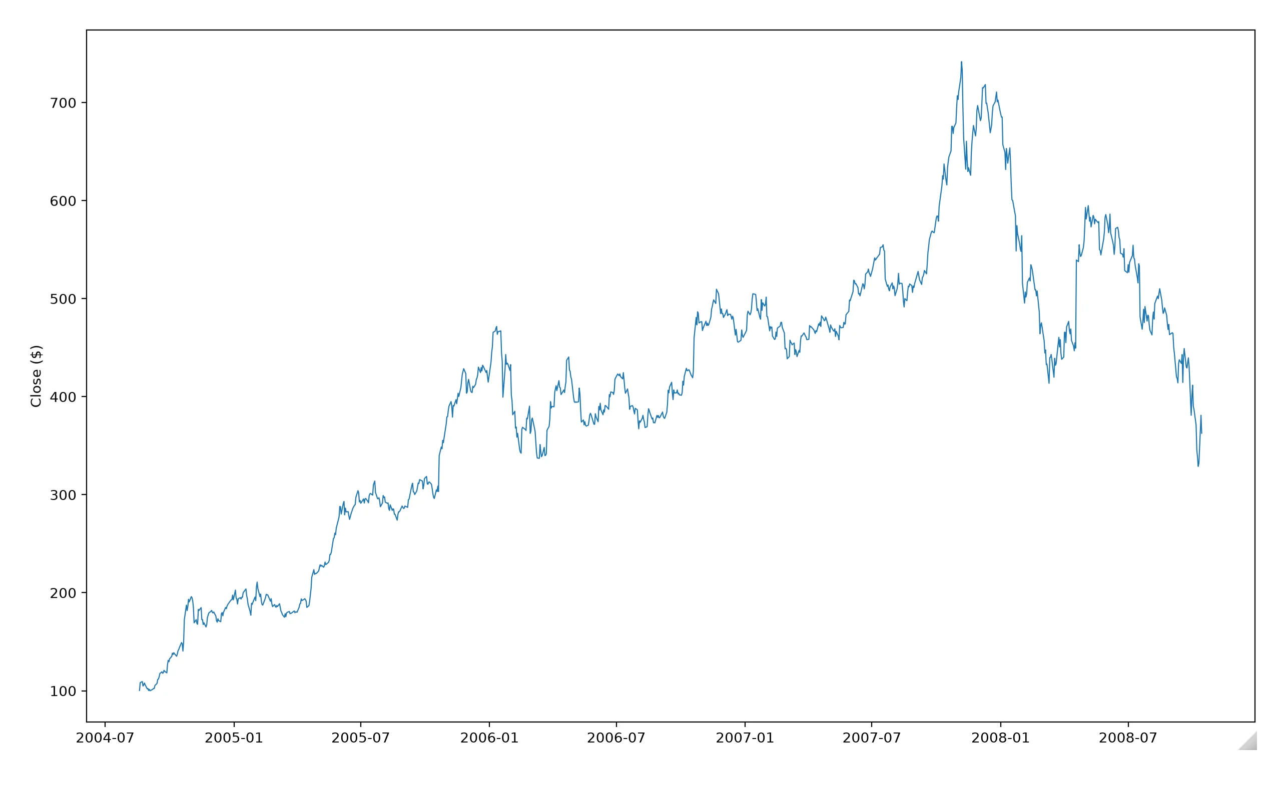
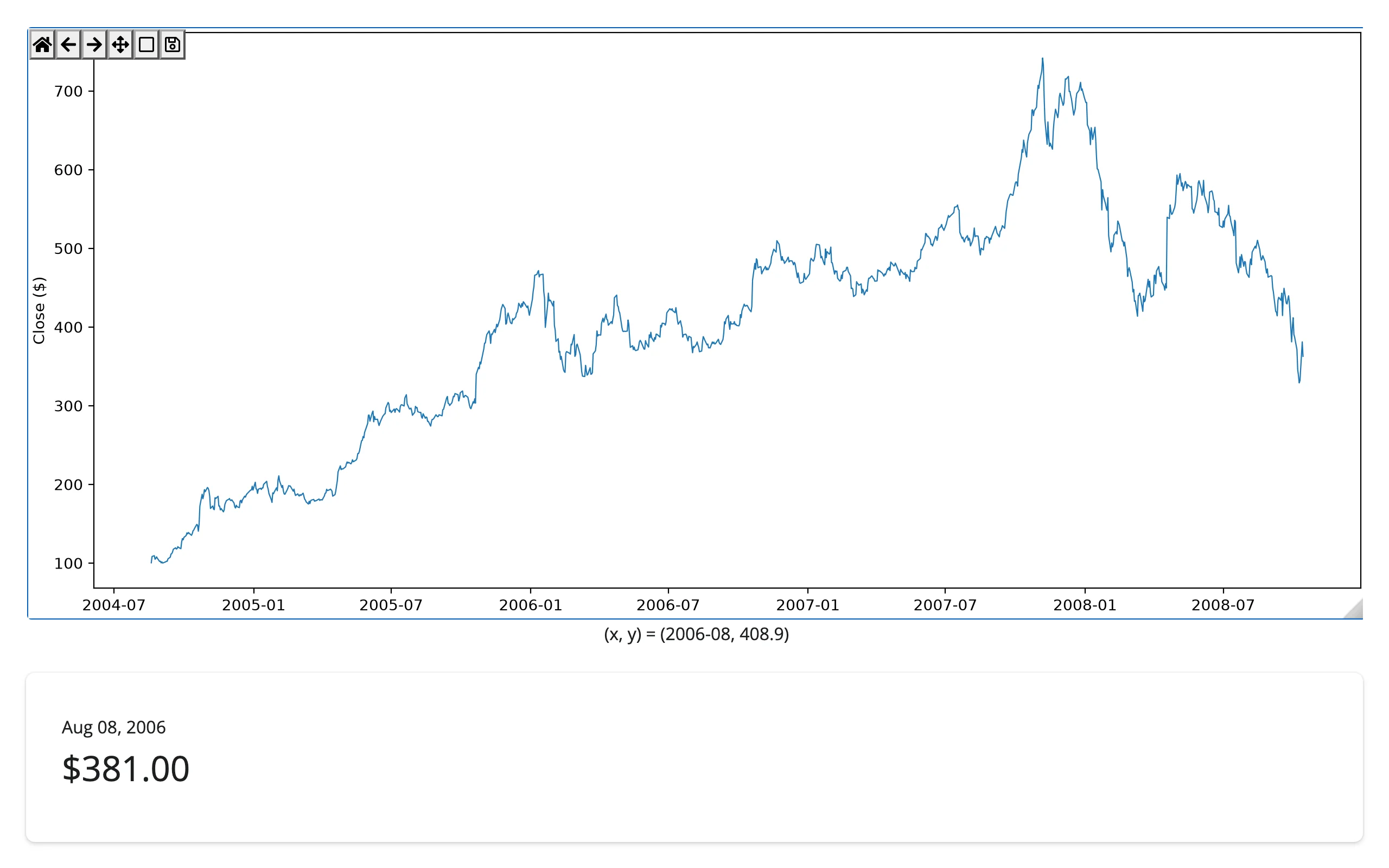
Click drives a detail card

examples/13_coordinate_click_detail.py33 lines

import numpy as np
from matplotlib.cbook import get_sample_data
from matplotlib.dates import date2num
from matplotlib.figure import Figure
from shiny import req
from shiny import ui as core_ui
from shiny.express import render, ui
from shinywidgets import render_matplotlib

ui.page_opts(fillable=True)

goog = get_sample_data("goog.npz")["price_data"]


@render_matplotlib
def plot():
    fig = Figure(layout="constrained")
    ax = fig.subplots()
    ax.plot(goog["date"], goog["close"], lw=0.8)
    ax.set_ylabel("Close ($)")
    return fig


@render.ui
def detail():
    ev = req(plot.clicked())
    i = int(
        np.clip(np.searchsorted(date2num(goog["date"]), ev.xdata), 0, len(goog) - 1)
    )
    date = goog["date"][i]
    return core_ui.value_box(
        f"{date.item().strftime('%b %d, %Y')}", f"${goog['close'][i]:.2f}"
    )

Note the from shiny import ui as core_ui import: Shiny Express’s own ui.value_box is a layout-time context manager with no return value, so a @render.ui function that needs to build and return a Tag uses the plain shiny.ui module instead.

Before click	After click

Box-select drives a filtered table

examples/14_coordinate_select_table.py46 lines

import numpy as np
import pandas as pd
from matplotlib.figure import Figure
from matplotlib.widgets import RectangleSelector
from shiny import reactive
from shiny.express import render, ui
from shinywidgets import render_matplotlib

ui.page_opts(fillable=True)

rng = np.random.default_rng(5)
cars = pd.DataFrame(
    {
        "model": [f"Car {i + 1}" for i in range(120)],
        "weight": rng.uniform(1.5, 5.0, 120).round(2),
    }
)
cars["mpg"] = (45 - 6 * cars["weight"] + rng.normal(0, 2.5, 120)).round(1)
selected = reactive.value(np.zeros(len(cars), dtype=bool))

with ui.layout_columns(col_widths=(7, 5)):

    @render_matplotlib
    def plot():
        fig = Figure(layout="constrained")
        ax = fig.subplots()
        points = ax.scatter(cars["weight"], cars["mpg"], alpha=0.7)
        ax.set_xlabel("Weight (1000 lbs)")
        ax.set_ylabel("Miles per gallon")

        def on_select(press, release):
            x0, x1 = sorted([press.xdata, release.xdata])
            y0, y1 = sorted([press.ydata, release.ydata])
            mask = cars["weight"].between(x0, x1) & cars["mpg"].between(y0, y1)
            points.set_facecolors(np.where(mask, "tab:orange", "tab:blue"))
            fig.canvas.draw_idle()
            selected.set(mask.to_numpy())

        fig._selector = RectangleSelector(ax, on_select, interactive=True)
        return fig

    with ui.card():

        @render.data_frame
        def table():
            return cars[selected()]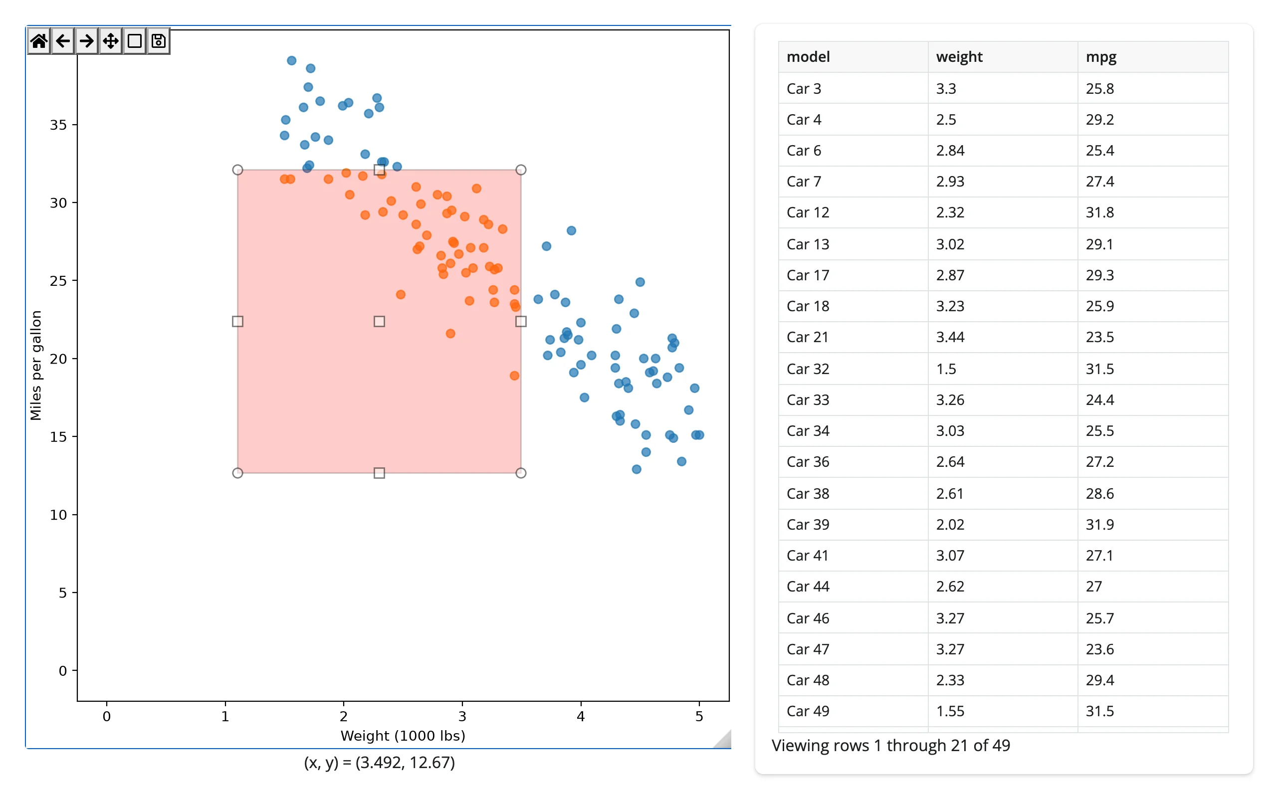

This pattern pairs well with itables or reactable in place of the plain @render.data_frame table, for sorting and paging in the selected subset.

Large data

@render_matplotlib has no large-data mode of its own: ipympl redraws the whole figure to a bitmap on every pan, zoom, or draw_idle() call, with no WebGL context and no server-side rasterization step. We didn’t re-measure a practical point-count ceiling this pass (the old evaluation’s panning-frame-rate numbers were dropped as stale). For a genuinely large series, either widget gets cheaper as data grows: Shiny’s own @render.plot (same matplotlib drawing underneath, a static PNG per render instead of a live canvas – see the introduction above), or a sibling built for scale, such as bokeh’s output_backend="webgl", plotly’s Scattergl, or datashader if the shape you want is a density raster. See Large data & performance for how those approaches compare.

Layout and sizing

examples/15_layout_sizing.py33 lines

import numpy as np
from matplotlib.figure import Figure
from shiny.express import ui
from shinywidgets import as_widget, render_matplotlib

ui.page_opts(fillable=True)

t = np.linspace(0, 10, 300)


def line_plot():
    fig = Figure(layout="constrained")
    ax = fig.subplots()
    ax.plot(t, np.sin(t))
    return fig


with ui.layout_columns():
    with ui.card(full_screen=True):
        ui.card_header("Fills its card (default)")

        @render_matplotlib
        def fills():
            return line_plot()

    with ui.card():
        ui.card_header("Explicit height, no footer")

        @render_matplotlib(height="220px", fillable=True)
        def fixed_height():
            canvas = as_widget(line_plot())
            canvas.footer_visible = False  # header is already hidden by default
            return canvas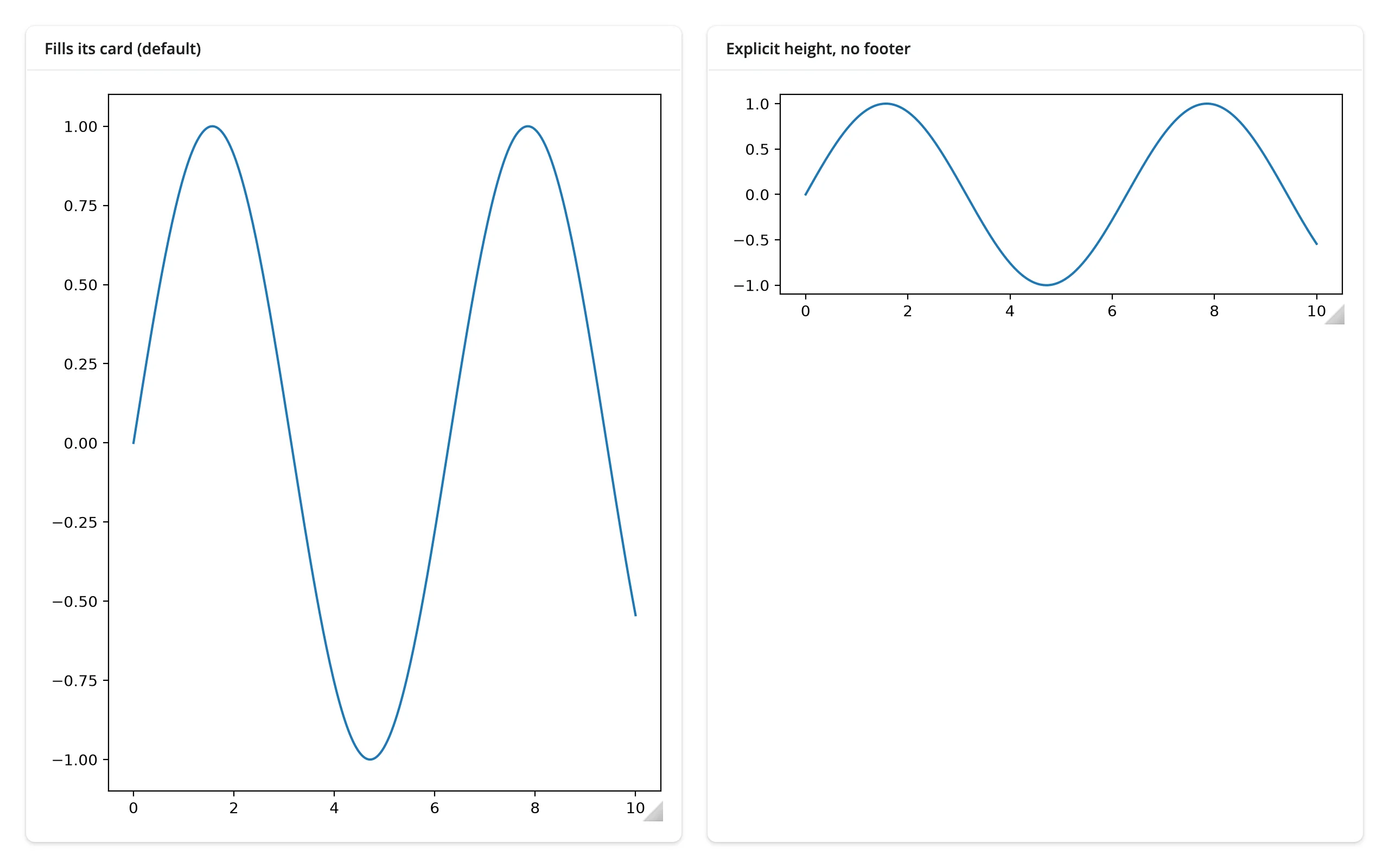

With no height (the default), the figure fills and resizes with its container, ignoring figsize. This is what you want inside a ui.card() or a fillable page.
With an explicit height, the figure keeps its figsize unless you also pass fillable=True – verified: without it, the figure silently renders at its full figsize regardless of the requested height, rather than being constrained to it. Pass both together to get a specific box size.
full_screen=True on the containing ui.card() works as expected; the figure re-fits when the card expands.
A coerced canvas’s “Figure N” header is hidden by default. If you want it back (e.g. to match a notebook screenshot), pass header_visible=True via as_widget(). The cursor-position footer stays visible by default; hide it the same way, with canvas.footer_visible = False, as above.

Gotchas and limitations

Everything below was verified on current main.

A zoom or pan tool stays active until you toggle it off. After dragging a zoom-to-rectangle or pan gesture, the toolbar button stays pressed; a plain click on the canvas is still treated as part of that gesture and clicked()/picked() don’t fire. Click the tool again (or Home) to return to normal click behavior. This is documented and intentional, but it’s an easy thing to trip over when testing your own app. Reading an .xlim/.ylim style accessor programmatically isn’t affected.
.read()/reactive_read() have nothing useful to read on the Canvas. Its synced traits are all chrome (header_visible, toolbar_position, pan_zoom_throttle, …) or private. Use the three accessors, or connect matplotlib’s own callbacks (fig.canvas.mpl_connect(...), ax.callbacks.connect(...)) for anything else. Scroll-to-zoom is off by default; set canvas.capture_scroll = True to enable it. Keyboard events need the figure focused (click it first).
An explicit height without fillable=True doesn’t constrain the figure. It renders at its default (or specified) figsize and simply doesn’t fit the requested box – see Layout and sizing.
Pyplot figures are closed automatically when rendered, the same way @render.plot closes its figure – so plt.subplots() is safe to use across sessions. Prefer Figure() or an explicit plt.subplots() over implicit current-figure idioms (plt.plot(), plt.gca(), a seaborn call without ax=) anyway: those are shared process-wide state, and a second concurrent session’s call can still interact with the first session’s figure before it’s closed.
A figure built under a GUI backend (Qt, Tk, the macOS backend) is supported, but warns. Its window is destroyed and ipympl’s canvas replaces it – a path that depends on platform-specific behavior the maintainers can’t test in CI. Build figures with Figure(), or select the agg backend before creating them (matplotlib.use("agg")), to avoid the warning entirely.
A draw-time error (e.g. invalid mathtext) shows as a normal output error, not a session crash – this includes both the first render and later in-place draw_idle() calls triggered from an effect.
No default layout engine. Without layout="constrained" (or a tight-layout call), labels can get clipped when the figure resizes to fill a card. The examples above all use Figure(layout="constrained") for this reason.
plotnine’s clicked() and limits() are the same underlying accessors as matplotlib’s (same AccessorSpec objects), but plotnine’s coordinates are in its transformed space (e.g. log10 under scale_x_log10()) and limits(ax) indexes facet panels. plotnine has no picked() – its geoms don’t expose matplotlib’s picker=. See the plotnine guide.

Gallery candidates

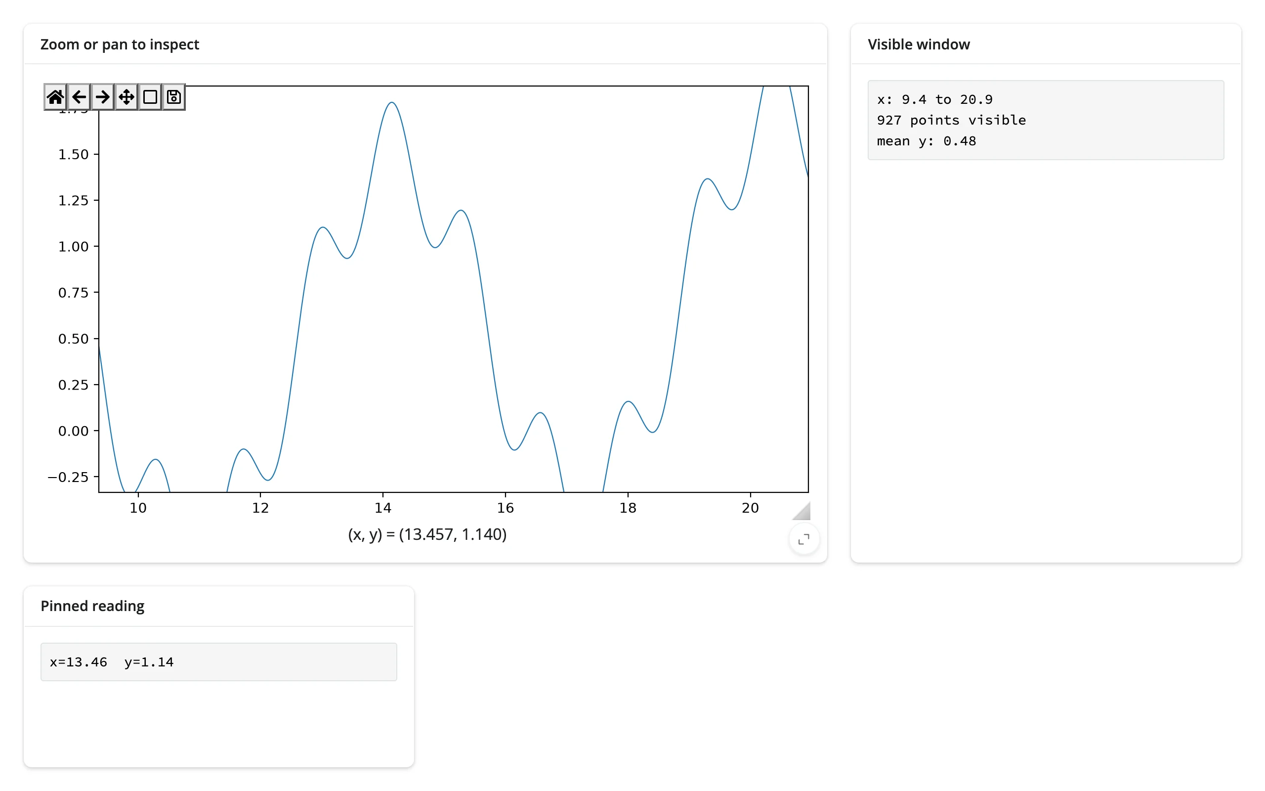
Template – gallery/template_zoom_and_click.py: a small, adaptable starting point combining limits() (a summary of the visible window) and clicked() (a pinned reading) on one synthetic signal. Swap in your own data and keep the two accessor-driven outputs.

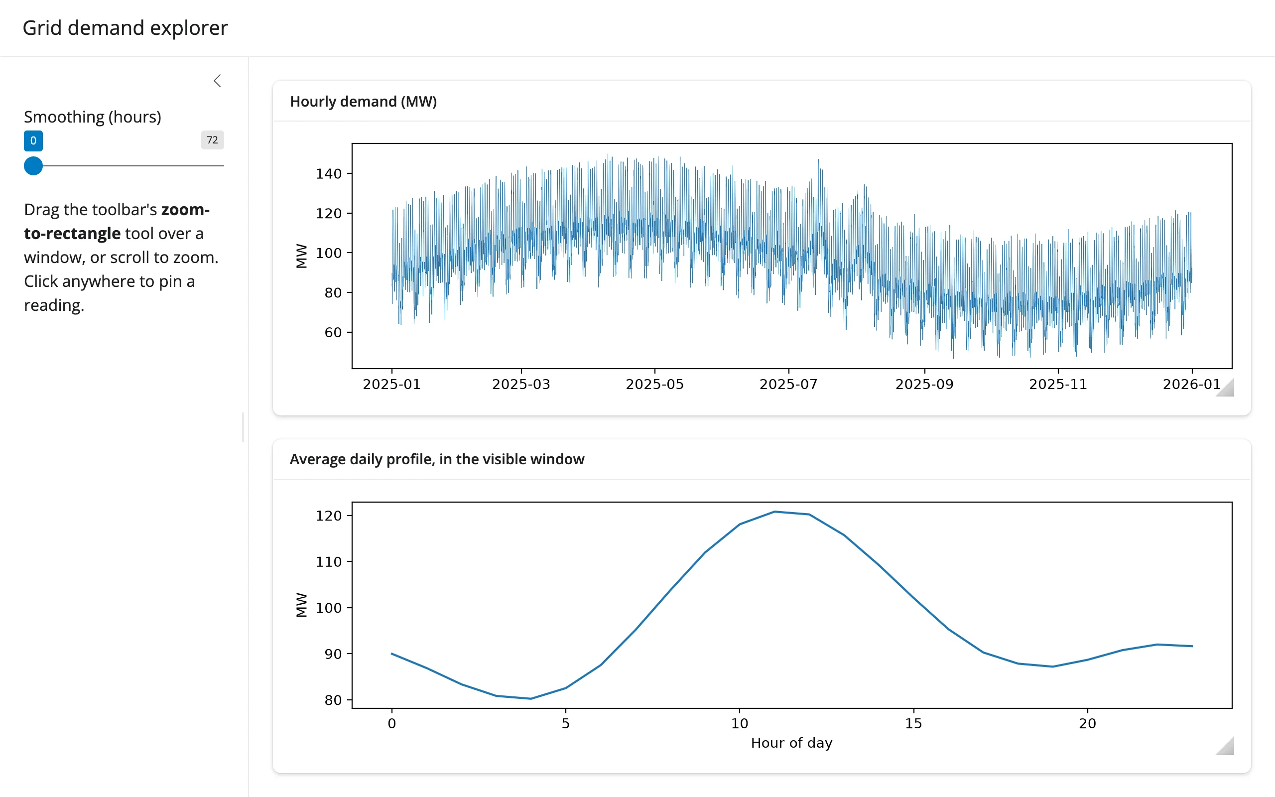
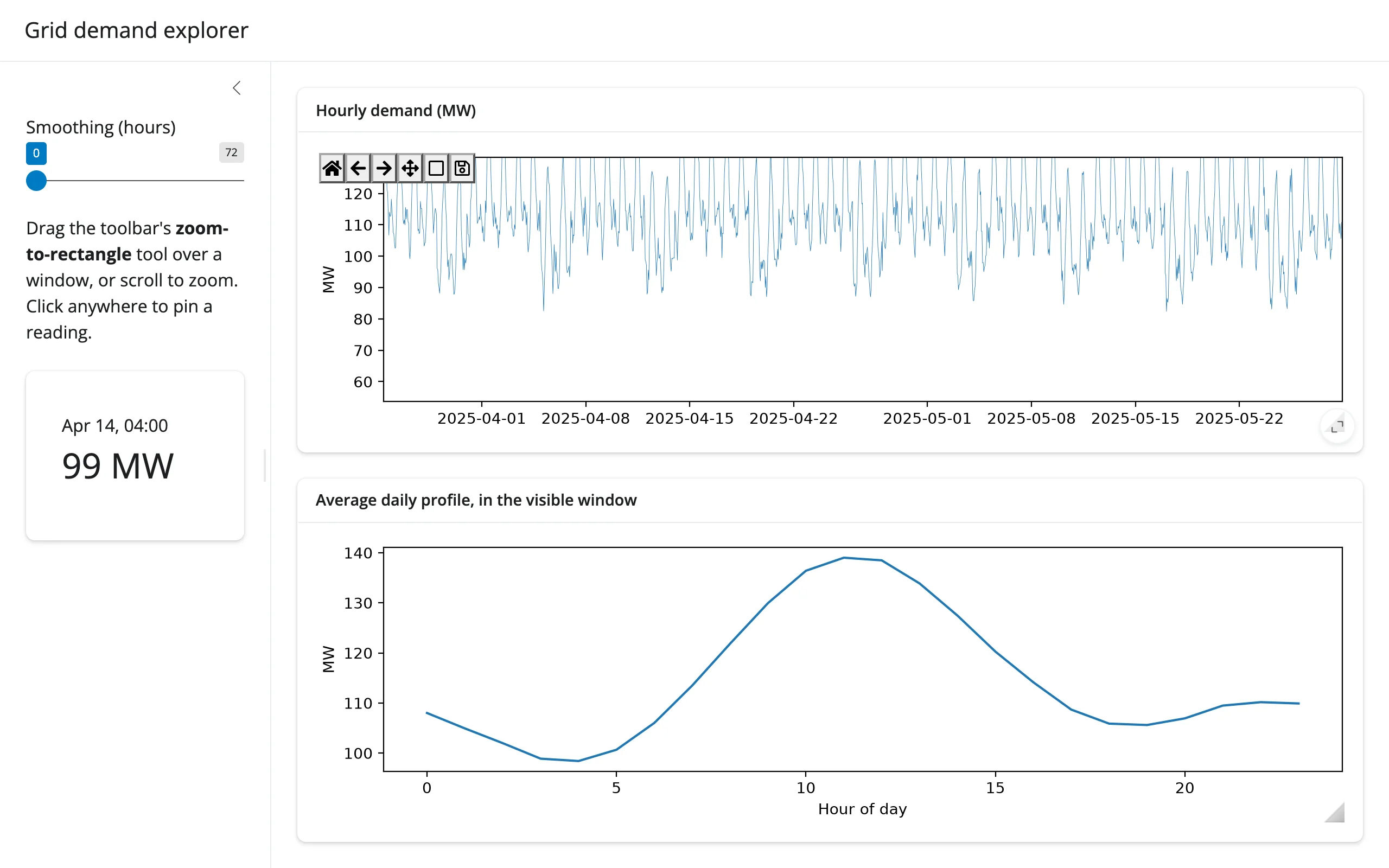
Showcase – gallery/showcase_grid_demand_explorer.py: a year of synthetic hourly power demand (a seasonal cycle, a daily double-peak, quiet weekends, two heat waves). Zooming the main chart redraws the daily-profile panel below it in place (limits() driving an effect that edits the panel’s line and rescales it); clicking pins the exact reading in the sidebar (clicked()); a smoothing slider restyles the main line in place without losing the zoom. The footer (cursor readout) is hidden on both plots; the header is already hidden by default.

Zoomed into a window, with a reading pinned:

Learn more

Matplotlib documentation
ipympl documentation
plotnine guide – grammar-of-graphics plots on the same ipympl engine, sharing clicked() and limits()
Shiny’s @render.plot – the static alternative, for cheaper, simpler, higher-concurrency apps