library(DBI)
library(dplyr)
library(tibble)
library(purrr)
library(glue)
library(cli)
library(sf)
library(ggplot2)

catalog <- Sys.getenv("DATABRICKS_CATALOG")
schema <- Sys.getenv("DATABRICKS_SCHEMA")

con <- dbConnect(
  odbc::databricks(),
  httpPath = Sys.getenv("DATABRICKS_PATH"),
  DefaultStringColumnLength = 65535
)

tbl_name <- function(table) {
  glue("{catalog}.{schema}.{table}")
}

per_station <- readRDS("per_station.rds")The spatial join
Stage three: putting the measurements and the places together
Draft. The code runs and the argument holds; the prose has not been copy-edited.
The station statistics from the last page have no geography on them. This page gives them one, by putting each station and each storm overflow inside a catchment, and it is the first point where the two connection paths stop being interchangeable.
Deciding which side to do it on
Both sides can do this. Databricks has spatial SQL, and sf is right here in the session. The choice is not about capability.
This example brings the geometry back and joins in sf, for three reasons worth stating because your situation may differ:
- The geometry is small. Four thousand catchment polygons is a few tens of megabytes, which is nothing.
- The result of the join feeds a bootstrap that has to run in R anyway, so the polygons have to arrive at some point regardless.
sfis the thing she already knows. Server-side spatial SQL is another dialect to learn for no gain at this size.
What the other route would cost, if your polygons were national coverage at full resolution rather than catchments: the geometry never enters the session, and you get back only the join keys. That is the right answer when the geometry is large and the result is small, which is the opposite of the case here.
Getting the polygons back at all
Geometry is stored as BINARY, and ODBC does not carry a BINARY column intact. That was established on Getting connected and finding the tables, and it decides the shape of the next few lines rather than being a footnote.
There are two ways around it. Encode server-side to text and decode here, which works over ODBC, or open a brickster connection and take the bytes directly. This page does the first, because the same query then works on either connection.
catchment_rows <- glue("
  SELECT
    water_body_id,
    water_body_name,
    ecological_class,
    overall_water_body_class,
    water_body_area_m2,
    base64(geom_wkb) AS geom_b64
  FROM {tbl_name('wfd_catchments')}
  WHERE geom_wkb IS NOT NULL
") |>
  dbGetQuery(conn = con) |>
  as_tibble()

nrow(catchment_rows)
[1] 4080Setting the CRS
WKB carries no SRID, so nothing in the bytes says which coordinate system they are in. sf will happily build geometry without one and every distance and area you compute afterwards will be wrong, silently.
The number has to come from you. These are British National Grid, EPSG:27700.
catchments <- catchment_rows$geom_b64 |>
  map(jsonlite::base64_dec) |>
  structure(class = "WKB") |>
  st_as_sfc(EWKB = FALSE, crs = 27700) |>
  st_sf(
    catchment_rows |> select(-geom_b64),
    geometry = _
  )

st_crs(catchments)$epsg
[1] 27700The check that this worked is not that it parsed. The catchment table carries its own area column, recorded before any of this, so the decoded geometry can be compared against something independent.
declared <- sum(catchments$water_body_area_m2, na.rm = TRUE)
measured <- sum(as.numeric(st_area(catchments)))
err <- abs(measured - declared) / declared

cli_alert_info(
  "area differs from declared by {round(100 * err, 4)}%"
)
ℹ area differs from declared by 0.0022%The two point layers
The overflows are longitude and latitude, which is a different CRS again. They have to be transformed before they can meet the catchments.
overflows <- glue("
  SELECT overflow_id, company, longitude, latitude
  FROM {tbl_name('storm_overflows')}
  WHERE longitude IS NOT NULL
    AND latitude IS NOT NULL
") |>
  dbGetQuery(conn = con) |>
  as_tibble() |>
  st_as_sf(
    coords = c("longitude", "latitude"),
    crs = 4326
  ) |>
  st_transform(27700)

nrow(overflows)
[1] 14190The stations are already easting and northing, so they need no transform, only a declaration of what they are.
stations <- glue("
  SELECT station_id, station_name, easting, northing
  FROM {tbl_name('hydrology_stations')}
  WHERE easting IS NOT NULL
    AND northing IS NOT NULL
") |>
  dbGetQuery(conn = con) |>
  as_tibble() |>
  st_as_sf(
    coords = c("easting", "northing"),
    crs = 27700
  )

nrow(stations)
[1] 9536Mixing these up is the classic failure, and it does not error. A longitude of -2 read as an easting of -2 metres puts the point in the sea off Africa, and the join simply matches nothing.
The join itself
overflow_catchment <- overflows |>
  st_join(catchments, join = st_within)

station_catchment <- stations |>
  st_join(catchments, join = st_within)
Checking the result is plausible
A join that matched nothing and a join that matched everything produce output of the same shape, so the count is the check.
matched <- sum(!is.na(overflow_catchment$water_body_id))

cli_alert_info(
  "{matched} of {nrow(overflows)} overflows fell inside \\
   a catchment ({round(100 * matched / nrow(overflows))}%)"
)
ℹ 13076 of 14190 overflows fell inside a catchment (92%)Not 100%, and that is the right answer rather than a problem. River catchments do not cover the coast, and an outfall that discharges to tidal water is genuinely outside all of them.
The eyeball check is worth the two lines it costs.
ggplot() +
  geom_sf(
    data = catchments,
    fill = "grey95",
    colour = NA
  ) +
  geom_sf(
    data = overflow_catchment,
    aes(colour = is.na(water_body_id)),
    size = 0.25,
    alpha = 0.6
  ) +
  scale_colour_manual(
    values = c("#447099", "#EE6331"),
    labels = c("in a catchment", "unmatched"),
    name = NULL
  ) +
  theme_void() +
  theme(legend.position = "bottom")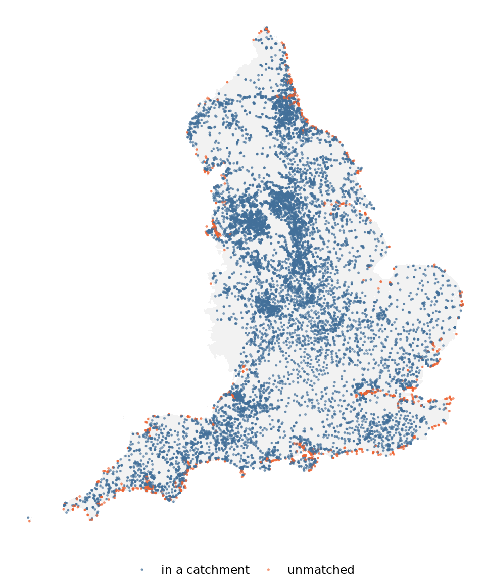
The unmatched points sit around the coastline, which is what should happen. Had they been scattered through the middle of the country, the CRS would be the first suspect.
Confirming the two sides agree
The join ran in sf. The same question can be put to the server, and the two answers should broadly agree. This is the check from Check that you get the same answer wherever it ran, applied to a spatial predicate rather than an aggregate.
The missing-SRID problem reappears here, on the other side of the wire. st_geomfromwkb() returns geometry with SRID 0 for exactly the reason sf needed a CRS argument, and the server refuses to compare SRID 0 against 27700 rather than guessing. st_setsrid() is what asserts it.
r_side <- overflow_catchment |>
  st_drop_geometry() |>
  filter(!is.na(water_body_id)) |>
  count(water_body_id, name = "n_r")

server_side <- glue("
  SELECT
    c.water_body_id,
    count(*) AS n_sql
  FROM {tbl_name('storm_overflows')} o
  JOIN {tbl_name('wfd_catchments')} c
    ON st_contains(
         -- st_setsrid is not optional: WKB carries no
         -- SRID, so st_geomfromwkb returns 0 and the
         -- server refuses to compare it against 27700.
         st_setsrid(st_geomfromwkb(c.geom_wkb), 27700),
         st_transform(
           st_point(o.longitude, o.latitude, 4326),
           27700
         )
       )
  GROUP BY c.water_body_id
") |>
  dbGetQuery(conn = con) |>
  as_tibble()

comparison <- full_join(
  r_side,
  server_side,
  by = "water_body_id"
)

comparison |>
  summarise(
    catchments = n(),
    agree = sum(n_r == n_sql, na.rm = TRUE),
    differ = sum(n_r != n_sql, na.rm = TRUE),
    total_r = sum(n_r, na.rm = TRUE),
    total_sql = sum(n_sql, na.rm = TRUE)
  )
# A tibble: 1 × 5
catchments agree differ total_r total_sql
<int> <int> <int> <int> <int64>
1 2638 2609 28 13076 13080The totals differ by a handful of points out of thirteen thousand. That is not a bug in either side: st_within and st_contains resolve a point sitting exactly on a shared boundary differently, and a catchment edge is shared by two polygons. It matters here only because it is the kind of difference worth expecting and quantifying rather than discovering later.
What goes forward
The analysis needs one row per catchment: how many overflows it contains, and what the flow variability of its stations looks like.
overflow_counts <- overflow_catchment |>
  st_drop_geometry() |>
  filter(!is.na(water_body_id)) |>
  count(water_body_id, name = "n_overflows")

station_flow <- station_catchment |>
  st_drop_geometry() |>
  filter(!is.na(water_body_id)) |>
  inner_join(per_station, by = "station_id") |>
  summarise(
    .by = water_body_id,
    n_stations = n(),
    median_cv = median(cv, na.rm = TRUE)
  )

catchment_panel <- catchments |>
  st_drop_geometry() |>
  select(
    water_body_id,
    water_body_name,
    ecological_class,
    water_body_area_m2
  ) |>
  left_join(overflow_counts, by = "water_body_id") |>
  inner_join(station_flow, by = "water_body_id") |>
  mutate(
    n_overflows = coalesce(n_overflows, 0L),
    area_km2 = water_body_area_m2 / 1e6,
    overflow_density = n_overflows / area_km2
  )

catchment_panel
# A tibble: 810 × 9
water_body_id water_body_name ecological_class water_body_area_m2 n_overflows
<chr> <chr> <chr> <dbl> <int>
1 GB1050350461… Jordan (East S… Good 25802596. 1
2 GB1020760710… Lowther (Lower) Not assessed 53512602. 5
3 GB1050310456… Jordan (Wellan… Bad 21338400 2
4 GB1060390302… Thame (Scotsgr… Moderate 89918004. 3
5 GB1060380279… Pymmes Brook u… Moderate 40778100 6
6 GB1120720717… Rawthey - Lower Good 16462406. 3
7 GB1070410124… Winterbourne S… Moderate 18353190. 0
8 GB1090540502… Platt Bk - sou… Moderate 25054100 0
9 GB1060390177… Caker Stream Bad 86218711. 0
10 GB1060390303… Thames (Leach … Poor 79293623. 2
# ℹ 800 more rows
# ℹ 4 more variables: n_stations <int>, median_cv <dbl>, area_km2 <dbl>,
# overflow_density <dbl>saveRDS(catchment_panel, "catchment_panel.rds")
saveRDS(catchments, "catchments.rds")
saveRDS(overflows, "overflows.rds")dbDisconnect(con)Next
Using the cores you already have.
This page rests on: catchment geometry is stored as BINARY and must be base64-encoded server-side to travel over ODBC; WKB carries no SRID, so the CRS must be supplied and is EPSG:27700 for this data; decoded catchment area agrees with the table’s declared area column to within thousandths of a percent; storm overflow locations are EPSG:4326 and need transforming before they will join; about 92% of overflows fall inside a river catchment, the remainder being coastal.