library(DBI)
library(dplyr)
library(dbplyr)
library(tibble)
library(glue)
library(cli)
library(sf)
library(ggplot2)

catalog <- Sys.getenv("DATABRICKS_CATALOG")
schema <- Sys.getenv("DATABRICKS_SCHEMA")

con <- dbConnect(
  odbc::databricks(),
  httpPath = Sys.getenv("DATABRICKS_PATH"),
  DefaultStringColumnLength = 65535
)

tbl_name <- function(table) {
  glue("{catalog}.{schema}.{table}")
}

wq_tbl <- function(table) {
  tbl(con, I(tbl_name(table)))
}Exploring and reducing the big table
Stage two: getting from tens of millions of rows to something you can hold
Draft. The code runs and the argument holds; the prose has not been copy-edited.
Thirty-two million rows go in and about a thousand come back. The whole of this page is about where that reduction happens, because it decides whether the analysis is possible at all.
Looking before reducing
Everything in this section is ordinary dplyr. None of it loads the table, and you can tell which by where collect() is: there isn’t one yet.
readings <- wq_tbl("hydrology_readings")
measures <- wq_tbl("hydrology_measures")
Start with the shape of the thing. This runs on the warehouse and returns three numbers.
readings |>
  summarise(
    rows = n(),
    first_day = min(date),
    last_day = max(date)
  ) |>
  collect()
Warning: Missing values are always removed in SQL aggregation functions.
Use `na.rm = TRUE` to silence this warning
This warning is displayed once every 8 hours.# A tibble: 1 × 3
rows first_day last_day
<int64> <date> <date>
1 32540721 2015-01-01 2024-12-30Ten years of daily data. Before trusting any of it, look at what the quality flag says, because a mean over unchecked values is not the mean you want.
readings |>
  count(quality, sort = TRUE) |>
  collect()
# A tibble: 5 × 2
quality n
<chr> <int64>
1 Good 26281624
2 Unchecked 3165682
3 Suspect 1665539
4 Estimated 1013873
5 Missing 414003About four fifths is Good. The rest is not junk, but it is not comparable either, and filtering to Good is a decision this analysis makes explicitly rather than by accident.
The readings table does not say what it is measuring. That lives on the measures table, which is small.
measures |>
  count(parameter_name, period_name, sort = TRUE) |>
  head(8) |>
  collect()
# A tibble: 8 × 3
parameter_name period_name n
<chr> <chr> <int64>
1 Level daily 5276
2 Dissolved Oxygen sub-daily 3807
3 Flow daily 3309
4 GroundwaterLevel <NA> 3095
5 Level 15min 2638
6 Temperature sub-daily 1948
7 Conductivity sub-daily 1942
8 PH sub-daily 1852A step that has to move
The analysis wants daily mean flow per station. The obvious way to write that is to filter the readings first and join afterwards, which is the wrong order:
readings |>
  filter(quality == "Good") |>
  inner_join(measures, by = join_by(measure == notation)) |>
  filter(parameter == "flow", period == 86400L)
That is not wrong in its answer, it is wrong in where the work lands. The join runs against every Good row in the table before anything narrows it to flow. Selecting the measures first means the join has roughly a thousand rows on one side instead of twenty-six million.
The rule generalises: filter the small side before the join, not the large side after it.
Reaching a function dbplyr will not translate
Picking daily mean flow needs a match on the end of value_statistic, and the natural R way to write that does not survive the trip:
filter(measures, grepl("mean", value_statistic))dbplyr translates a great deal, and grepl() is not part of it. The query reaches the server with grepl still in it and fails there, not here, with UNRESOLVED_ROUTINE. That is the signature of a translation gap rather than a mistake in your logic.
The escape hatch is dplyr::sql(), which passes a fragment through untouched. You are writing Spark SQL at that point, so the dialect is theirs and not R’s.
flow_measures <- measures |>
  filter(
    parameter == "flow",
    period == 86400L,
    sql("value_statistic LIKE '%/mean'")
  )

flow_measures |>
  summarise(measures = n()) |>
  collect()
# A tibble: 1 × 1
measures
<int64>
1 1103Where the line falls in this pipeline
Here is the whole reduction, with the one line that matters marked. Everything above collect() runs on Databricks; everything below runs in your session.
per_station <- readings |>
  inner_join(
    flow_measures,
    by = join_by(measure == notation)
  ) |>
  filter(
    quality == "Good",
    !is.na(value),
    value >= 0
  ) |>
  summarise(
    .by = station_id,
    n_days = n(),
    mean_flow = mean(value, na.rm = TRUE),
    sd_flow = sd(value, na.rm = TRUE)
  ) |>
  filter(n_days >= 1000) |>
  # <== everything above this line ran on Databricks
  collect() |>
  mutate(cv = sd_flow / mean_flow)

per_station
# A tibble: 1,029 × 5
station_id n_days mean_flow sd_flow cv
<chr> <int64> <dbl> <dbl> <dbl>
1 8a2f47f1-711e-4805-8536-a49bfda4d06c 3632 0.652 0.904 1.39
2 8b07239d-fb98-4f27-b182-def7799b6c34_2044 3608 0.970 0.928 0.957
3 962530ad-afe9-49e5-8fcd-33af504efdf6 3520 0.160 0.0728 0.454
4 a9417599-e466-4b53-babe-0c81229c4328 3454 4.32 5.30 1.23
5 7ca88e3b-d821-4093-951e-1ecd25e78ef5 3201 0.285 0.497 1.74
6 a97cc80d-f8dd-4fa9-a0db-482ab1b41f71 3373 0.318 0.235 0.739
7 bce8bf9b-9b67-4bee-9c90-3c7f65c3444e 2912 0.975 0.833 0.854
8 b9933a62-f326-4d77-9206-ebb335161831 3092 21.2 23.5 1.11
9 88be649b-6ea9-4daa-b81b-7767cbc5b995 1564 0.00309 0.000753 0.243
10 977e3ab5-ec6e-4040-acf2-8a178818a5c8 3285 0.288 0.296 1.03
# ℹ 1,019 more rowsThe mutate() sits below the line deliberately. It could run either side, and putting it in the session keeps the SQL to the part that has to be SQL.
n_days >= 1000 drops stations with less than about three years of record. That is a judgement about what a variability estimate is worth, not a technical constraint.
It is worth seeing what that judgement costs, because a filter on record length could quietly have been a filter on geography. It is not: the stations that survive are thinned out of the whole network rather than taken from one part of it.
The coordinates are eastings and northings on the British National Grid (EPSG 27700), so coord_sf() is given that CRS explicitly rather than left to infer one. Stating it is the habit worth copying: a map drawn from unprojected latitude and longitude is stretched north to south at this latitude, and nothing warns you.
# station_xy.rds carries easting and northing for every station, from the
# same query [Joining tables that do not share a key](spatial.qmd) uses.
station_xy <- readRDS("station_xy.rds") |>
  st_as_sf(coords = c("easting", "northing"), crs = 27700) |>
  mutate(kept = station_id %in% per_station$station_id)

ggplot(station_xy) +
  geom_sf(data = ~filter(.x, !kept), colour = "#CFCFCF", size = 0.35) +
  geom_sf(data = ~filter(.x, kept), colour = "#447099", size = 0.5) +
  coord_sf(crs = 27700, datum = 27700) +
  theme_void(base_size = 11)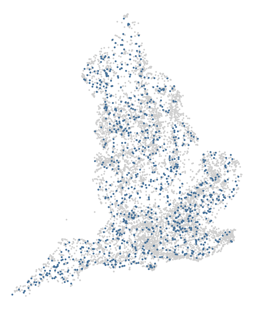
What came back
cli_alert_info(
  "{nrow(per_station)} stations, \\
   {round(as.numeric(object.size(per_station)) / 1024)} KB"
)
ℹ 1029 stations, 138 KBThirty-two and a half million rows became about a thousand, and a few hundred kilobytes. Everything after this page is ordinary R on an ordinary data frame.
The coefficient of variation is the number the rest of the example uses. A station with a CV near zero has a steady flow; a high CV means a river that is mostly low and occasionally in flood.
per_station |>
  summarise(
    median_cv = median(cv, na.rm = TRUE),
    min_cv = min(cv, na.rm = TRUE),
    max_cv = max(cv, na.rm = TRUE)
  )
# A tibble: 1 × 3
median_cv min_cv max_cv
<dbl> <dbl> <dbl>
1 1.12 0.0878 3.09Checking the reduction against the server
The count came back as a single number, so it is worth confirming that number was computed over what you think it was.
server_side <- readings |>
  inner_join(
    flow_measures,
    by = join_by(measure == notation)
  ) |>
  filter(quality == "Good", !is.na(value), value >= 0) |>
  summarise(
    rows = n(),
    stations = n_distinct(station_id)
  ) |>
  collect()

server_side
# A tibble: 1 × 2
rows stations
<int64> <int64>
1 3239134 1066The station count here is higher than the thousand-odd that came back, and that difference is the n_days >= 1000 filter rather than anything going wrong.
saveRDS(per_station, "per_station.rds")dbDisconnect(con)Next
This page rests on: the readings table holds about 32.5 million rows spanning 2015 to 2024; roughly 80% of readings carry quality Good; grepl() has no Spark SQL translation and fails server-side with UNRESOLVED_ROUTINE, so dplyr::sql() is needed to match on value_statistic; filtering the measures table before the join rather than the readings table after it is what keeps the join small; the reduction yields about a thousand stations and a few hundred kilobytes.