library(dplyr)
library(tibble)
library(purrr)
library(glue)
library(cli)
library(parallel)
library(ggplot2)
library(bit64)

per_station <- readRDS("per_station.rds")
source("R/setup.R")
n_cores <- wq_cores()Simulating from a summary
Stage five: a thousand parameter draws per station, on the cores you have
Draft. The code runs and the argument holds; the prose has not been copy-edited.
The first simulation in this example, and the one that does not need a cluster. It is the ordinary shape: the data shrank server-side, what came back is a summary, and the expensive part is repeating a small computation many times over that summary.
What is being simulated, and why
The question is how often a station’s daily flow drops below a low-flow threshold, and how uncertain that number is given only ten years of record.
The threshold is a property of the station: the tenth percentile of its own fitted flow distribution, so it is a low flow for that river rather than a number carried over from a larger one. That much a single fit gives you. What a single fit does not give you is how much to trust it, because the mean and standard deviation behind it were themselves estimated from a finite record, and a station with three years of readings pins them down less well than one with ten.
So the uncertainty that matters here is uncertainty in the fitted parameters. Each draw perturbs the fitted mean and standard deviation by their own sampling error, then asks what fraction of a year would fall below the threshold under those perturbed parameters. A thousand such draws give a thousand answers, and their spread is the interval. Stations with a longer record get a tighter one, which is the whole point.
Two honest caveats. The sampling error used below is the textbook approximation for a normal fit, applied to a lognormal fitted from a mean and a standard deviation rather than from the readings themselves, so it is rough. And this is a demonstration of mechanism, not a hydrological finding: the distributional choice is convenient rather than defended.
The summary the simulation runs on
Everything needed is already in the session, and it is small.
sim_input <- per_station |>
  filter(
    !is.na(mean_flow),
    !is.na(sd_flow),
    mean_flow > 0,
    sd_flow > 0
  ) |>
  select(station_id, n_days, mean_flow, sd_flow, cv) |>
  mutate(n_days = as.integer(n_days))

nrow(sim_input)
[1] 1029n_days arrives as an integer64, which is how a Spark BIGINT lands in R. It has to be converted before it is used in arithmetic, and the conversion needs bit64 attached: without it, as.integer() on one of these columns returns zero and as.numeric() returns a number around 1e-320, both silently. That is why library(bit64) is in the setup chunk. The record length is about to become part of the answer, so a column of zeros here would not error, it would just quietly remove the thing the stage is measuring.
Fitting the distribution
Daily flow is positive and right-skewed, so a lognormal is the obvious first reach. Its two parameters follow from the mean and standard deviation already computed server-side, which means no second pass over the readings.
lognormal_pars <- function(mean_x, sd_x) {
  sigma2 <- log1p((sd_x / mean_x)^2)
  list(
    meanlog = log(mean_x) - sigma2 / 2,
    sdlog = sqrt(sigma2)
  )
}

sim_input <- sim_input |>
  mutate(
    pars = map2(mean_flow, sd_flow, lognormal_pars),
    meanlog = map_dbl(pars, "meanlog"),
    sdlog = map_dbl(pars, "sdlog")
  ) |>
  select(-pars)

sim_input |>
  select(station_id, mean_flow, sd_flow, meanlog, sdlog)
# A tibble: 1,029 × 5
station_id mean_flow sd_flow meanlog sdlog
<chr> <dbl> <dbl> <dbl> <dbl>
1 8a2f47f1-711e-4805-8536-a49bfda4d06c 0.652 0.904 -0.964 1.04
2 8b07239d-fb98-4f27-b182-def7799b6c34_2044 0.970 0.928 -0.356 0.806
3 962530ad-afe9-49e5-8fcd-33af504efdf6 0.160 0.0728 -1.92 0.433
4 a9417599-e466-4b53-babe-0c81229c4328 4.32 5.30 1.00 0.958
5 7ca88e3b-d821-4093-951e-1ecd25e78ef5 0.285 0.497 -1.95 1.18
6 a97cc80d-f8dd-4fa9-a0db-482ab1b41f71 0.318 0.235 -1.36 0.660
7 bce8bf9b-9b67-4bee-9c90-3c7f65c3444e 0.975 0.833 -0.299 0.740
8 b9933a62-f326-4d77-9206-ebb335161831 21.2 23.5 2.65 0.896
9 88be649b-6ea9-4daa-b81b-7767cbc5b995 0.00309 0.000753 -5.81 0.240
10 977e3ab5-ec6e-4040-acf2-8a178818a5c8 0.288 0.296 -1.61 0.851
# ℹ 1,019 more rowsThe unit of work
One station, one function, returning one row. Nothing in it knows how it will be called, which is the property that lets the same function run serially, across cores, or on a cluster.
simulate_station <- function(station_id,
                             meanlog,
                             sdlog,
                             n_days,
                             threshold_q = 0.1,
                             n_draws = 1000,
                             days_per_year = 365) {
  set.seed(strtoi(substr(rlang::hash(station_id), 1, 7), 16L))

  # The threshold comes from the fit as it stands, not from a perturbed
  # version of it, so it stays a fixed low-flow level for this station
  # while the draws move around it.
  threshold <- qlnorm(threshold_q, meanlog, sdlog)

  # Sampling error of the two fitted parameters, given n_days of record.
  se_meanlog <- sdlog / sqrt(n_days)
  se_sdlog <- sdlog / sqrt(2 * n_days)

  rate <- map_dbl(seq_len(n_draws), \(i) {
    days_per_year * plnorm(
      threshold,
      rnorm(1, meanlog, se_meanlog),
      rnorm(1, sdlog, se_sdlog)
    )
  })

  tibble(
    station_id = station_id,
    n_days = n_days,
    threshold = threshold,
    mean_days = mean(rate),
    lower = quantile(rate, 0.025, names = FALSE),
    upper = quantile(rate, 0.975, names = FALSE)
  )
}
Each draw asks what share of a year falls below the threshold under one perturbed version of the fit, rather than dealing out 365 individual days and counting them. Both are defensible, and this one is chosen deliberately: counting days adds the coin-flip noise of a single year to every draw, and at these record lengths that noise is several times larger than the parameter uncertainty, so it would bury the signal the stage exists to show. Asking for the share isolates the part that answers the question.
Serially first
The version that is slow and obviously correct, kept because everything after it has to agree with it. This is the version to debug, not a stepping stone to be discarded.
small <- sim_input |> slice_head(n = 50)

serial_time <- system.time(
  serial_result <- small |>
    pmap(\(station_id, meanlog, sdlog, n_days, ...) {
      simulate_station(station_id, meanlog, sdlog, n_days)
    }) |>
    list_rbind()
)

serial_result
# A tibble: 50 × 6
station_id n_days threshold mean_days lower upper
<chr> <int> <dbl> <dbl> <dbl> <dbl>
1 8a2f47f1-711e-4805-8536-a49bfda4d06c 3632 0.101 36.5 33.9 39.3
2 8b07239d-fb98-4f27-b182-def7799b6c34_… 3608 0.249 36.5 33.6 39.3
3 962530ad-afe9-49e5-8fcd-33af504efdf6 3520 0.0838 36.6 33.7 39.7
4 a9417599-e466-4b53-babe-0c81229c4328 3454 0.799 36.5 33.9 39.3
5 7ca88e3b-d821-4093-951e-1ecd25e78ef5 3201 0.0312 36.5 33.6 39.5
6 a97cc80d-f8dd-4fa9-a0db-482ab1b41f71 3373 0.110 36.5 33.5 39.4
7 bce8bf9b-9b67-4bee-9c90-3c7f65c3444e 2912 0.287 36.5 33.3 39.5
8 b9933a62-f326-4d77-9206-ebb335161831 3092 4.50 36.5 33.5 39.6
9 88be649b-6ea9-4daa-b81b-7767cbc5b995 1564 0.00221 36.6 32.5 40.9
10 977e3ab5-ec6e-4040-acf2-8a178818a5c8 3285 0.0673 36.6 33.8 39.5
# ℹ 40 more rowsAcross the cores you have
The change from the serial version is one line: pmap() becomes an mclapply() over the same function. Using the cores you already have settled why it is parallel here rather than furrr.
run_all <- function(input, cores) {
  rows <- seq_len(nrow(input))

  mclapply(rows, mc.cores = cores, FUN = \(i) {
    simulate_station(
      input$station_id[i],
      input$meanlog[i],
      input$sdlog[i],
      input$n_days[i]
    )
  }) |>
    list_rbind()
}

parallel_time <- system.time(
  sim_result <- run_all(sim_input, n_cores)
)

nrow(sim_result)
[1] 1029The two runs are not the same size, so they are not comparable as timings. Both are single runs in a session with 1 core available, quoted so the numbers mean something rather than as a benchmark.
tibble(
  run = c(
    glue("serial, {nrow(small)} stations"),
    glue("mclapply, {nrow(sim_input)} stations")
  ),
  seconds = c(
    serial_time[["elapsed"]],
    parallel_time[["elapsed"]]
  )
)
# A tibble: 2 × 2
run seconds
<chr> <dbl>
1 serial, 50 stations 0.369
2 mclapply, 1029 stations 6.10 The parallel run has to agree with the serial one on the stations they share. That check is worth making explicitly, because a parallel run that silently reorders or drops rows looks exactly like one that did not.
Agreeing on the numbers is the easy half, and on its own it proves less than it appears to: the seed is derived from the station id, so any run that reaches a given station at all computes the same value for it, whatever order the work arrived in. The half that can actually fail is whether every station came back exactly once. So the check below reorders the serial input before re-running it, then compares the set of ids and the row count as well as the values.
shuffled <- small |> arrange(desc(station_id))

reordered_result <- shuffled |>
  pmap(\(station_id, meanlog, sdlog, n_days, ...) {
    simulate_station(station_id, meanlog, sdlog, n_days)
  }) |>
  list_rbind()

comparison <- serial_result |>
  select(station_id, serial = mean_days) |>
  inner_join(
    sim_result |> select(station_id, par = mean_days),
    by = "station_id"
  )

ids_match <- setequal(reordered_result$station_id, serial_result$station_id)
counts_match <- nrow(reordered_result) == nrow(serial_result) &&
  !anyDuplicated(sim_result$station_id)
rows_joined <- nrow(comparison) == nrow(serial_result)
max_diff <- max(abs(comparison$serial - comparison$par))

stopifnot(
  "reordering changed which stations came back" = ids_match,
  "a station was dropped or duplicated" = counts_match,
  "the parallel run did not cover every serial station" = rows_joined
)

cli_alert_info(
  "{nrow(comparison)} stations compared, \\
   max difference {signif(max_diff, 3)}"
)
ℹ 50 stations compared, max difference 0The result
sim_result |>
  arrange(desc(mean_days)) |>
  slice_head(n = 8)
# A tibble: 8 × 6
station_id n_days threshold mean_days lower upper
<chr> <int> <dbl> <dbl> <dbl> <dbl>
1 3cdb0ed3-0644-45f1-b6fb-7c1944578bf6 1284 0.0325 36.7 31.9 41.4
2 efe53bb2-d752-4aa6-af43-e2240eae3675 3318 0.186 36.7 33.6 39.7
3 05d216a3-0102-43d8-9907-d7698b32eb03 1098 0.0222 36.7 31.5 42.1
4 2ec6d59e-e3c9-453d-9c1b-2ea1fcf4d6d9 3100 0.0458 36.7 33.8 39.7
5 4d9c0d31-89d2-4330-994c-1376cdcb56c6 2098 0.217 36.7 32.9 40.4
6 69c693b6-12ef-43bc-a20e-74160a53350d 1921 0.0169 36.7 32.9 40.6
7 39b9499d-25bb-46e5-83d6-5c97a39b9bdb 1955 0.163 36.7 32.8 40.5
8 a45c1d4d-e45e-417b-a0f0-83867ff5926d 1258 0.0173 36.6 32.0 41.6The central estimate is near 36.5 days for every station, and that is arithmetic rather than a result: the threshold is each station’s own tenth percentile, so a tenth of a year is the answer by construction. The number that carries information is the width of the interval around it.
sim_result |>
  mutate(width = upper - lower) |>
  ggplot(aes(n_days, width)) +
  geom_point(alpha = 0.3, colour = "#447099") +
  labs(
    x = "days of record behind the fit",
    y = "width of the 95% interval (days)"
  ) +
  theme_minimal(base_size = 11)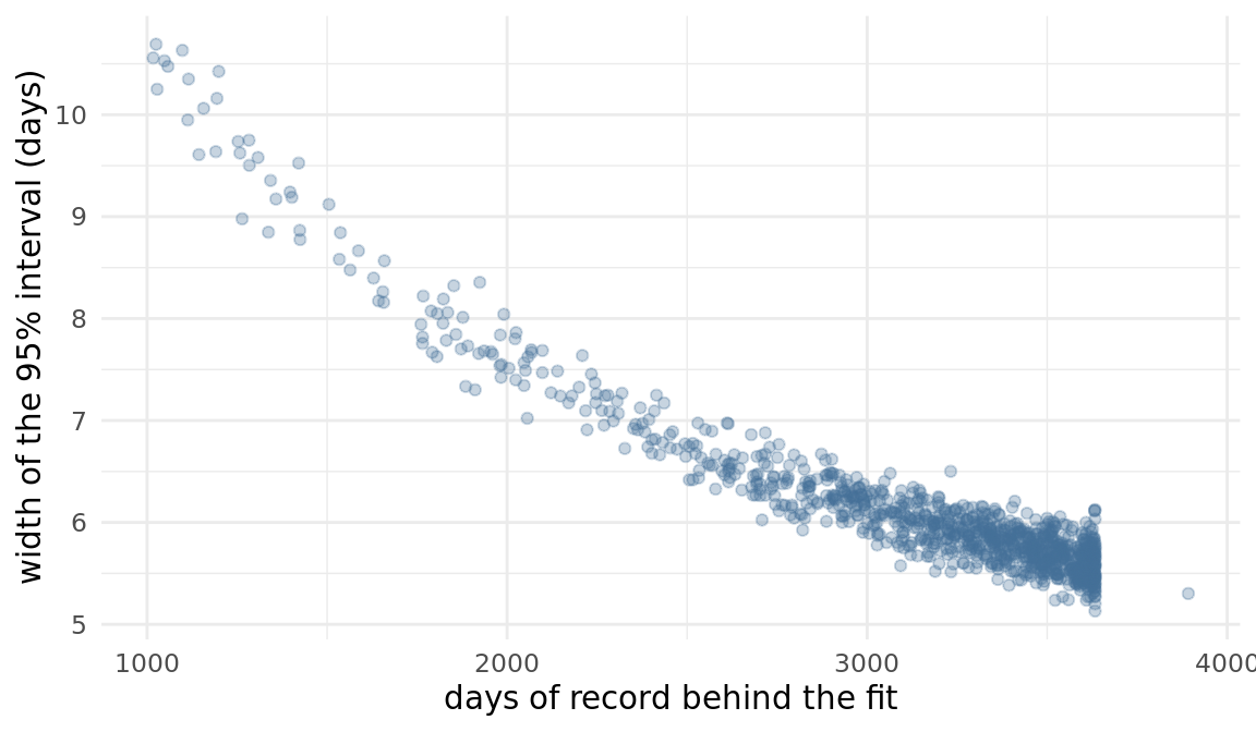
That is the shape a sampling-error argument predicts, and seeing it is the check that the stage is measuring what it claims to. A station with three years of record carries roughly twice the uncertainty of one with ten.
This one is finished
The honest checkpoint. The page reaches it and stops, rather than reaching for the cluster to complete a demonstration.
The arithmetic is small: about a thousand stations, a thousand parameter draws each. That finishes on a handful of cores in a time that does not justify starting anything, and the correct thing to do is nothing further.
Saying so is what earns the credibility for the next page, where the answer is different.
When this shape does need the cluster
The example’s own simulation is small. The shape is not inherently small, and yours may not be.
The arithmetic rather than a threshold, because the threshold depends on your machine: the number of independent units, the cost of one unit, and the cores you can reach in your own session. When the product of the first two outgrows the third by enough that the run stops fitting in a working day, the same code moves to cluster compute with the unit of work unchanged.
Two things carry over unchanged, and both matter for the next page:
- The worker function is the same function. It takes its arguments and returns a data frame, and nothing about it knows where it is running.
- The backend inside the worker changes, because
furrris not there.parallel::mclapply()is.
What does not carry over is the assumption that distributing is free. On a single-node cluster, R in one session using mclapply() was more than twice as fast as distributing the same work, because distribution costs serialisation and there were no other machines to spread onto. Reaching for the cluster when there is nothing to distribute to is slower than not reaching for it.
The trap in expressing it the natural way
Worth carrying here even though the cluster is not used on this page, because it is the mistake made at exactly the moment this code first moves across.
The unit of work is naturally a station, so group_by looks like the way to say that. It is not: it collapses the job to a single R process and runs slower for an identical answer, and on a current runtime it does not run at all. Partition instead, and let each worker loop over the stations in its slice. Run a Monte Carlo simulation carries the detail.
saveRDS(sim_result, "sim_result.rds")Next
When the simulation carries the geometry, which is the same shape with one thing added, and the addition is what changes the answer.
This page rests on: per-station mean and standard deviation of daily flow are sufficient to parameterise a lognormal without a second pass over the readings; the count of days behind each fit is available in the same summary, so the sampling error of those two parameters can be formed without returning to the readings either; about a thousand stations at a thousand draws each finishes on a handful of local cores; on a single-node cluster parallel::mclapply() in one cluster-side session was over twice as fast as spark_apply() for the same draws; spark_apply(group_by =) uses one R process where the partition path uses several, runs slower for an identical answer, and fails outright on rpy2 3.6.x.