Shiny makes it easy to create rich, interactive experiences in pure Python with a fully reactive framework. No JavaScript required!
Shiny Express
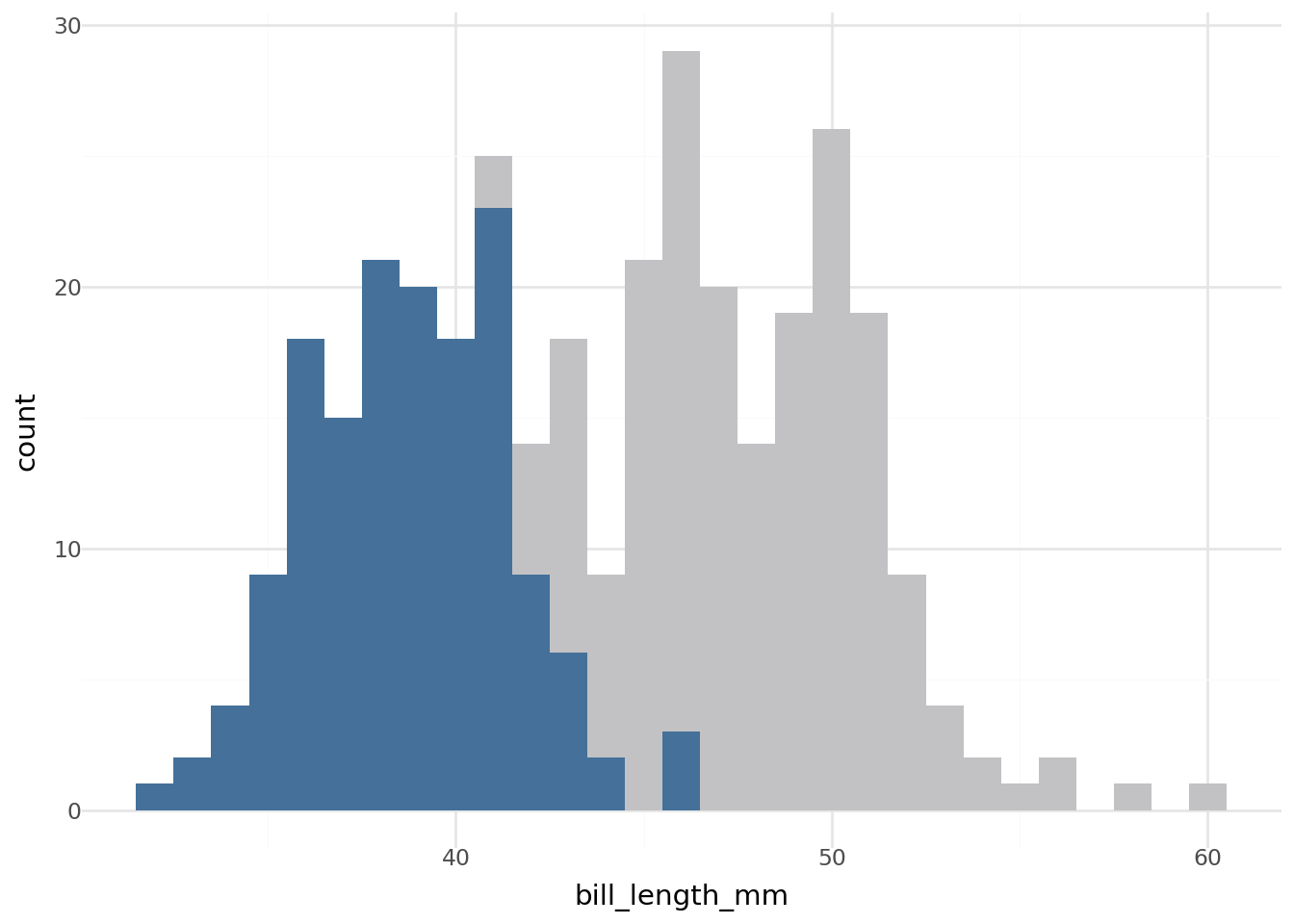
Here’s the Shiny application we’ll be creating. Give it a try! See how the different penguin distributions compare to one another.
#| '!! shinylive warning !!': |
#|   shinylive does not work in self-contained HTML documents.
#|   Please set `embed-resources: false` in your metadata.
#| standalone: true
#| components: [viewer]
#| viewerHeight: 500

from palmerpenguins import load_penguins
from plotnine import aes, geom_histogram, ggplot, theme_minimal
from shiny.express import input, render, ui

dat = load_penguins()
species = dat["species"].unique().tolist()

ui.input_radio_buttons("species", "Species", species, inline=True)


@render.plot
def plot():
    sel = dat[dat["species"] == input.species()]
    return (
        ggplot(aes(x="bill_length_mm"))
        + geom_histogram(dat, fill="#C2C2C4", binwidth=1)
        + geom_histogram(sel, fill="#447099", binwidth=1)
        + theme_minimal()
    )
Goal
Let’s create a simple shiny application that uses the palmerpenguins dataset and visualizes it using plotnine.
We’ll use shiny to give us interactive radio buttons to change what species of the bill_length_mm variable we will want to highlight.
Prototype
We’ll be using palmerpenguins for the dataset, and plotnine to visualize the palmer penguin’s bill_length_mm column as a histogram.
from palmerpenguins import load_penguinsdat = load_penguins()dat.head()
species
island
bill_length_mm
bill_depth_mm
flipper_length_mm
body_mass_g
sex
year
0
Adelie
Torgersen
39.1
18.7
181.0
3750.0
male
2007
1
Adelie
Torgersen
39.5
17.4
186.0
3800.0
female
2007
2
Adelie
Torgersen
40.3
18.0
195.0
3250.0
female
2007
3
Adelie
Torgersen
NaN
NaN
NaN
NaN
NaN
2007
4
Adelie
Torgersen
36.7
19.3
193.0
3450.0
female
2007
Here’s the base code we’ll be starting with. It creates 2 histograms layerd on top of one another. The base layer is the distribution of all the penguin species. and the blue layer on top will the distribution of the selected penguin species.
To learn more about how the plotting code works in plotnine, take a look at our plotnine lab.
Wouldn’t it be nice if we could have something to toggle between one of the 3 penguin species instead of having us manually change the species variable and re-run our code?
Now we’re ready for a Shiny dashboard! All we need is some mechanism to list and provide the options for the user to pass into the species variable. Then pandas can filter the selected layer data, and plotnine can render the new data layer.
Shiny Express
Shiny Express is designed to make it significantly easier to get started with Shiny, and to write simple apps with a minimum of boilerplate.
Wherever you write your UI or output code, is where it will render in the application. In this sense Shiny Express is similar to Streamlit. If you’re looking for syntax where the UI and outputs are separated, similar to Dash, then take a look at the Shiny Core Lab.
User interface
Before we get all components reacting to one another, let’s start with mapping out how our application will look.
id: this is what shiny uses to reference the value selected by the input (more on this later).
label: the text the user will see by the component.
choices: the options our radio button component will display to the user and value it will use in code.
#| '!! shinylive warning !!': |
#|   shinylive does not work in self-contained HTML documents.
#|   Please set `embed-resources: false` in your metadata.
# | standalone: true
# | components: [editor, viewer]
# | layout: horizontal
from shiny.express import ui

ui.input_radio_buttons(
    id="species",
    label="Species",
    choices=["Adelie", "Gentoo", "Chinstrap"],
)
Run your shiny application
In Positron or VSCode, assuming you have the VSCode Shiny Extension installed, create a file named app.py, copy + paste the code above and hit the play button to run your application.
Or you can go to https://shinylive.io/py and copy + paste the code there and run your application.
Let’s have the buttons run horizontally to take up less space. We can use the inline=True to change the orientation of the radio buttons.
#| '!! shinylive warning !!': |
#|   shinylive does not work in self-contained HTML documents.
#|   Please set `embed-resources: false` in your metadata.
# | standalone: true
# | components: [editor, viewer]
# | layout: horizontal
from shiny.express import ui

ui.input_radio_buttons(
    id="species",
    label="Species",
    choices=["Adelie", "Gentoo", "Chinstrap"],
    inline=True,
)
Output component
Now let’s add all that data and plotting code from earlier into our application.
If we just dump in our code, the application errors because it does not know what to do with the figure that’s trying to be printed.
from shiny.express import uifrom palmerpenguins import load_penguinsfrom plotnine import aes, geom_histogram, ggplot, theme_minimalui.input_radio_buttons(id="species", label="Species", choices=["Adelie", "Gentoo", "Chinstrap"], inline=True,)dat = load_penguins()species ="Adelie"sel = dat.loc[dat.species == species]# this will cause a TypeError: Invalid tag item type( ggplot(aes(x="bill_length_mm"))+ geom_histogram(dat, fill="#C2C2C4", binwidth=1)+ geom_histogram(sel, fill="#447099", binwidth=1)+ theme_minimal())
In shiny, each output needs to be wrapped in it’s own function, and the corresponding output decorator applied to the function so Shiny knows how to render the output.
For example, we want to return a plot, so we will need to wrap our plotnine code, and decorate it with the @render.plot decorator.
#| '!! shinylive warning !!': |
#|   shinylive does not work in self-contained HTML documents.
#|   Please set `embed-resources: false` in your metadata.
# | standalone: true
# | components: [editor, viewer]
# | layout: horizontal
from shiny.express import ui, render

from palmerpenguins import load_penguins
from plotnine import aes, geom_histogram, ggplot, theme_minimal

ui.input_radio_buttons(
    id="species",
    label="Species",
    choices=["Adelie", "Gentoo", "Chinstrap"],
    inline=True,
)

dat = load_penguins()
species = "Adelie"
sel = dat.loc[dat.species == species]

@render.plot
def plot():
    return (
        ggplot(aes(x="bill_length_mm"))
        + geom_histogram(dat, fill="#C2C2C4", binwidth=1)
        + geom_histogram(sel, fill="#447099", binwidth=1)
        + theme_minimal()
    )
Return your values
Don’t forget to return the object you want displayed in the function! Otherwise the output will not render.
Make it reactive
Great! We have our input component, we have our output component, all we need to do now is connect the value selected by the input component and have the output react to the selected input.
First, when we are working with linking input and output values, they must all exist in the same “reactive context”, i.e., be in a function that is decorated by shiny, in our case all our code that needs to react needs to be in the function that is decorated by @render.plot.
#| '!! shinylive warning !!': |
#|   shinylive does not work in self-contained HTML documents.
#|   Please set `embed-resources: false` in your metadata.
# | standalone: true
# | components: [editor, viewer]
# | layout: horizontal
from shiny.express import ui, render

from palmerpenguins import load_penguins
from plotnine import aes, geom_histogram, ggplot, theme_minimal

ui.input_radio_buttons(
    id="species",
    label="Species",
    choices=["Adelie", "Gentoo", "Chinstrap"],
    inline=True,
)

dat = load_penguins()

@render.plot
def plot():
    species = "Adelie"
    sel = dat.loc[dat.species == species]

    return (
        ggplot(aes(x="bill_length_mm"))
        + geom_histogram(dat, fill="#C2C2C4", binwidth=1)
        + geom_histogram(sel, fill="#447099", binwidth=1)
        + theme_minimal()
    )
Now we’re ready to link the input and output components together. We now need to import the input object from shiny. The input object keep track of all the input components in the application and allows you to access the input value by the id we used when we created the input component.
In our example, our input_radio_buttons() input component was given an id="species", so we can access the value in the radio button by using input.species(). Here we have to add round parenthesis to the value, because we’re trying to get the actual value stored in the species input.
Don’t forget the round parenthesis ()!
Don’t forget to add a set of round parenthesis, () when you are trying to get the value of a component. You need to “call” it for Shiny to compute its value. This is how we work with reactivity in shiny, and this prevents us from writing callbacks in our application.
Instead of hard-coding species = "Adelie", we can replace it with species = input.species(), and it will return the value from our radio button input component.
#| '!! shinylive warning !!': |
#|   shinylive does not work in self-contained HTML documents.
#|   Please set `embed-resources: false` in your metadata.
# | standalone: true
# | components: [editor, viewer]
# | layout: horizontal
from shiny.express import ui, render, input

from palmerpenguins import load_penguins
from plotnine import aes, geom_histogram, ggplot, theme_minimal

ui.input_radio_buttons(
    id="species",
    label="Species",
    choices=["Adelie", "Gentoo", "Chinstrap"],
    inline=True,
)

dat = load_penguins()

@render.plot
def plot():
    species = input.species()
    sel = dat.loc[dat.species == species]

    return (
        ggplot(aes(x="bill_length_mm"))
        + geom_histogram(dat, fill="#C2C2C4", binwidth=1)
        + geom_histogram(sel, fill="#447099", binwidth=1)
        + theme_minimal()
    )
Our final application
After tidying up the code a bit, here’s our final Shiny application!
If you want you can tinker with the code and run the application right in the browser, or copy + paste the code and run it in your IDE.
#| '!! shinylive warning !!': |
#|   shinylive does not work in self-contained HTML documents.
#|   Please set `embed-resources: false` in your metadata.
#| standalone: true
#| components: [editor, viewer]
#| layout: horizontal
#| viewerHeight: 500

from palmerpenguins import load_penguins
from plotnine import aes, geom_histogram, ggplot, theme_minimal
from shiny.express import input, render, ui

dat = load_penguins()
species = dat["species"].unique().tolist()

ui.input_radio_buttons("species", "Species", species, inline=True)


@render.plot
def plot():
    sel = dat[dat["species"] == input.species()]
    return (
        ggplot(aes(x="bill_length_mm"))
        + geom_histogram(dat, fill="#C2C2C4", binwidth=1)
        + geom_histogram(sel, fill="#447099", binwidth=1)
        + theme_minimal()
    )