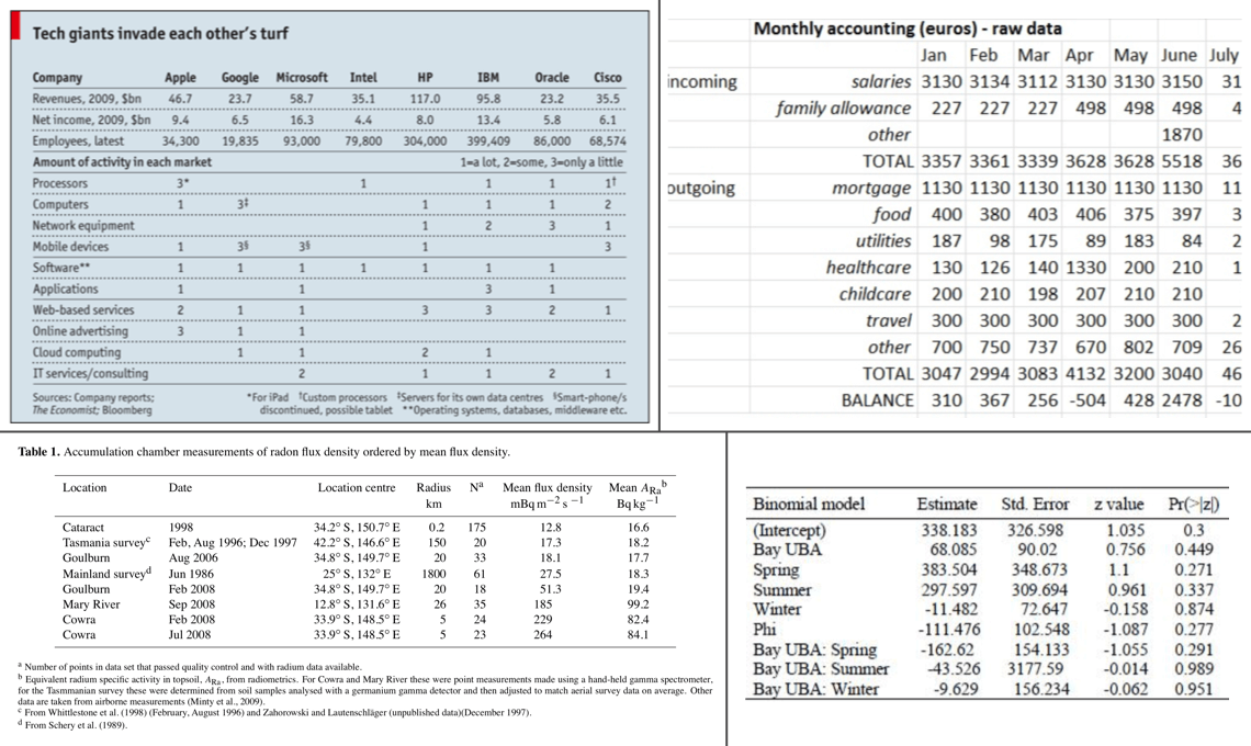
 We can think of display tables as output only, where we'd not want to use them as input ever again. Other features include annotations, table element styling, and text transformations that serve to communicate the subject matter more clearly.
# Let's Install
The installation really couldn't be much easier. Use this:
``` bash
pip install great_tables
```
Once installed, you are ready to build your first table.
# A Basic Table using **Great Tables**
> **Note: Note**
>
> The example below requires the Pandas library to be installed. But Pandas is not required to use Great Tables. You can also use a Polars DataFrame.
Let's use a subset of the `islands` dataset available within `great_tables.data`:
``` python
from great_tables import GT, md, html
from great_tables.data import islands
islands_mini = islands.head(10)
```
The `islands` data is a simple **Pandas** DataFrame with 2 columns and that'll serve as a great start. Speaking of which, the main entry point into the **Great Tables** API is the [GT](../reference/GT.md#great_tables.GT) class. Let's use that to make a presentable table:
``` python
# Create a display table showing ten of the world's largest islands
gt_tbl = GT(islands_mini)
# Show the output table
gt_tbl
```
| name | size |
|--------------|-------|
| Africa | 11506 |
| Antarctica | 5500 |
| Asia | 16988 |
| Australia | 2968 |
| Axel Heiberg | 16 |
| Baffin | 184 |
| Banks | 23 |
| Borneo | 280 |
| Britain | 84 |
| Celebes | 73 |
That doesn't look too bad! Sure, it's basic but we really didn't really ask for much. We did receive a proper table with column labels and the data. Oftentimes however, you'll want a bit more: a **Table header**, a **Stub**, and sometimes *source notes* in the **Table Footer** component.
> **Note: Note**
>
> Typically we use Great Tables in an notebook environment or within a Quarto document. Tables won't print to the console, but using the [show()](../reference/GT.show.md#great_tables.GT.show) method on a table object while in the console will open the HTML table in your default browser.
# **Polars** DataFrame support
[GT](../reference/GT.md#great_tables.GT) accepts both **Pandas** and **Polars** DataFrames. You can pass a **Polars** DataFrame to [GT](../reference/GT.md#great_tables.GT), or use its `DataFrame.style` property.
``` python
import polars as pl
df_polars = pl.from_pandas(islands_mini)
# Approach 1: call GT ----
GT(df_polars)
# Approach 2: Polars style property ----
df_polars.style
```
| name | size |
|--------------|-------|
| Africa | 11506 |
| Antarctica | 5500 |
| Asia | 16988 |
| Australia | 2968 |
| Axel Heiberg | 16 |
| Baffin | 184 |
| Banks | 23 |
| Borneo | 280 |
| Britain | 84 |
| Celebes | 73 |
> **Note: Note**
>
> The `polars.DataFrame.style` property is currently considered [unstable](https://docs.pola.rs/api/python/stable/reference/dataframe/style.html#polars.DataFrame.style), and may change in the future. Using [GT](../reference/GT.md#great_tables.GT) on a **Polars** DataFrame will always work.
# Some Beautiful Examples
In the following pages we'll use **Great Tables** to turn DataFrames into beautiful tables, like the ones below.
Show the Code
``` python
from great_tables import GT, md, html
from great_tables.data import islands
islands_mini = islands.head(10)
(
GT(islands_mini, rowname_col = "name")
.tab_header(
title="Large Landmasses of the World",
subtitle="The top ten largest are presented"
)
.tab_source_note(
source_note="Source: The World Almanac and Book of Facts, 1975, page 406."
)
.tab_source_note(
source_note=md("Reference: McNeil, D. R. (1977) *Interactive Data Analysis*. Wiley.")
)
.tab_stubhead(label="landmass")
)
```
We can think of display tables as output only, where we'd not want to use them as input ever again. Other features include annotations, table element styling, and text transformations that serve to communicate the subject matter more clearly.
# Let's Install
The installation really couldn't be much easier. Use this:
``` bash
pip install great_tables
```
Once installed, you are ready to build your first table.
# A Basic Table using **Great Tables**
> **Note: Note**
>
> The example below requires the Pandas library to be installed. But Pandas is not required to use Great Tables. You can also use a Polars DataFrame.
Let's use a subset of the `islands` dataset available within `great_tables.data`:
``` python
from great_tables import GT, md, html
from great_tables.data import islands
islands_mini = islands.head(10)
```
The `islands` data is a simple **Pandas** DataFrame with 2 columns and that'll serve as a great start. Speaking of which, the main entry point into the **Great Tables** API is the [GT](../reference/GT.md#great_tables.GT) class. Let's use that to make a presentable table:
``` python
# Create a display table showing ten of the world's largest islands
gt_tbl = GT(islands_mini)
# Show the output table
gt_tbl
```
| name | size |
|--------------|-------|
| Africa | 11506 |
| Antarctica | 5500 |
| Asia | 16988 |
| Australia | 2968 |
| Axel Heiberg | 16 |
| Baffin | 184 |
| Banks | 23 |
| Borneo | 280 |
| Britain | 84 |
| Celebes | 73 |
That doesn't look too bad! Sure, it's basic but we really didn't really ask for much. We did receive a proper table with column labels and the data. Oftentimes however, you'll want a bit more: a **Table header**, a **Stub**, and sometimes *source notes* in the **Table Footer** component.
> **Note: Note**
>
> Typically we use Great Tables in an notebook environment or within a Quarto document. Tables won't print to the console, but using the [show()](../reference/GT.show.md#great_tables.GT.show) method on a table object while in the console will open the HTML table in your default browser.
# **Polars** DataFrame support
[GT](../reference/GT.md#great_tables.GT) accepts both **Pandas** and **Polars** DataFrames. You can pass a **Polars** DataFrame to [GT](../reference/GT.md#great_tables.GT), or use its `DataFrame.style` property.
``` python
import polars as pl
df_polars = pl.from_pandas(islands_mini)
# Approach 1: call GT ----
GT(df_polars)
# Approach 2: Polars style property ----
df_polars.style
```
| name | size |
|--------------|-------|
| Africa | 11506 |
| Antarctica | 5500 |
| Asia | 16988 |
| Australia | 2968 |
| Axel Heiberg | 16 |
| Baffin | 184 |
| Banks | 23 |
| Borneo | 280 |
| Britain | 84 |
| Celebes | 73 |
> **Note: Note**
>
> The `polars.DataFrame.style` property is currently considered [unstable](https://docs.pola.rs/api/python/stable/reference/dataframe/style.html#polars.DataFrame.style), and may change in the future. Using [GT](../reference/GT.md#great_tables.GT) on a **Polars** DataFrame will always work.
# Some Beautiful Examples
In the following pages we'll use **Great Tables** to turn DataFrames into beautiful tables, like the ones below.
Show the Code
``` python
from great_tables import GT, md, html
from great_tables.data import islands
islands_mini = islands.head(10)
(
GT(islands_mini, rowname_col = "name")
.tab_header(
title="Large Landmasses of the World",
subtitle="The top ten largest are presented"
)
.tab_source_note(
source_note="Source: The World Almanac and Book of Facts, 1975, page 406."
)
.tab_source_note(
source_note=md("Reference: McNeil, D. R. (1977) *Interactive Data Analysis*. Wiley.")
)
.tab_stubhead(label="landmass")
)
```
| Large Landmasses of the World | |
|---|---|
| The top ten largest are presented | |
| landmass | size |
| Africa | 11506 |
| Antarctica | 5500 |
| Asia | 16988 |
| Australia | 2968 |
| Axel Heiberg | 16 |
| Baffin | 184 |
| Banks | 23 |
| Borneo | 280 |
| Britain | 84 |
| Celebes | 73 |
| Source: The World Almanac and Book of Facts, 1975, page 406. | |
| Reference: McNeil, D. R. (1977) Interactive Data Analysis. Wiley. | |
| New York Air Quality Measurements | ||||||
|---|---|---|---|---|---|---|
| Daily measurements in New York City (May 1-10, 1973) | ||||||
| Time | Measurement | |||||
| Year | Month | Day | Ozone, ppbV |
Solar R., cal/m2 |
Wind, mph |
Temp, °F |
| 1973 | 5 | 1 | 41.0 | 190.0 | 7.4 | 67 |
| 1973 | 5 | 2 | 36.0 | 118.0 | 8.0 | 72 |
| 1973 | 5 | 3 | 12.0 | 149.0 | 12.6 | 74 |
| 1973 | 5 | 4 | 18.0 | 313.0 | 11.5 | 62 |
| 1973 | 5 | 5 | 14.3 | 56 | ||
| 1973 | 5 | 6 | 28.0 | 14.9 | 66 | |
| 1973 | 5 | 7 | 23.0 | 299.0 | 8.6 | 65 |
| 1973 | 5 | 8 | 19.0 | 99.0 | 13.8 | 59 |
| 1973 | 5 | 9 | 8.0 | 19.0 | 20.1 | 61 |
| 1973 | 5 | 10 | 194.0 | 8.6 | 69 | |
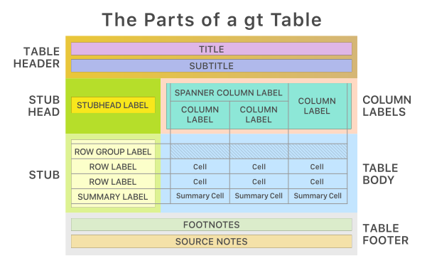 The following list describes each major component of a **Great Tables** output, ordered from top to bottom:
- the **Table Header** (optional; with a **title** and possibly a **subtitle**)
- the **Stub** and the **Stub Head** (optional; contains *row labels*, optionally within *row groups* having *row group labels*)
- the **Column Labels** (contains *column labels*, optionally under *spanner labels*)
- the **Table Body** (contains *columns* and *rows* of *cells*)
- the **Table Footer** (optional; possibly with one or more **source notes**)
Each of these parts is covered in detail throughout the rest of this User Guide. The pages that follow will show you how to add a header and footer, create a stub with row labels and groupings, organize your column labels with spanners, format cell values, and apply styling to any part of the table.
The following list describes each major component of a **Great Tables** output, ordered from top to bottom:
- the **Table Header** (optional; with a **title** and possibly a **subtitle**)
- the **Stub** and the **Stub Head** (optional; contains *row labels*, optionally within *row groups* having *row group labels*)
- the **Column Labels** (contains *column labels*, optionally under *spanner labels*)
- the **Table Body** (contains *columns* and *rows* of *cells*)
- the **Table Footer** (optional; possibly with one or more **source notes**)
Each of these parts is covered in detail throughout the rest of this User Guide. The pages that follow will show you how to add a header and footer, create a stub with row labels and groupings, organize your column labels with spanners, format cell values, and apply styling to any part of the table.